
Chapter 13
Excel power
In this chapter, you will:
List all files in a folder
Import data from a CSV file
Learn methods of splitting and merging data
Export data to an XML file
Create a log file
Clean a report so you can analyze the data
Learn favorite techniques of various VBA pros
A major secret of successful programmers is to never waste time writing the same code twice. They all have little bits—or even big bits—of code that they use over and over again. Another big secret is to never take 8 hours doing something that can be done in 10 minutes—which is what this book is about!
This chapter contains programs donated by several Excel power programmers. These are programs they have found useful and that they hope will help you, too. Not only can these programs save you time, but they also can teach you new ways of solving common problems.
Different programmers have different programming styles, and we didn’t rewrite the submissions. As you review the code in this chapter, you’ll notice different ways of doing the same task, such as referring to ranges.
File operations
The utilities shown in the following sections deal with handling files in folders. Being able to loop through a list of files in a folder is a useful task.
Listing files in a directory
This utility was submitted by our good friend Nathan P. Oliver of Minneapolis, Minnesota.
This program returns the file name, size, and date modified of all specified file types in the selected directory and its subfolders:
Sub ExcelFileSearch()
Dim srchExt As Variant, srchDir As Variant
Dim i As Long, j As Long, strName As String
Dim varArr(1 To 1048576, 1 To 3) As Variant
Dim strFileFullName As String
Dim ws As Worksheet
Dim fso As Object

Let srchExt = Application.InputBox("Please Enter File Extension", "Info Request")
If srchExt = False And Not TypeName(srchExt) = "String" Then
      Exit Sub
End If

Let srchDir = BrowseForFolderShell
If srchDir = False And Not TypeName(srchDir) = "String" Then
    Exit Sub
End If
Application.ScreenUpdating = False
Set ws = ThisWorkbook.Worksheets.Add(Sheets(1))
On Error Resume Next
Application.DisplayAlerts = False
ThisWorkbook.Worksheets("FileSearch Results").Delete
Application.DisplayAlerts = True
On Error GoTo 0
ws.Name = "FileSearch Results"

Let strName = Dir$(srchDir & "*" & srchExt)
Do While strName <> vbNullString
     Let i = i + 1
     Let strFileFullName = srchDir & strName
     Let varArr(i, 1) = strFileFullName
     Let varArr(i, 2) = FileLen(strFileFullName)  1024
     Let varArr(i, 3) = FileDateTime(strFileFullName)
     Let strName = Dir$()
Loop

Set fso = CreateObject("Scripting.FileSystemObject")
Call recurseSubFolders(fso.GetFolder(srchDir), varArr(), i, CStr(srchExt))
Set fso = Nothing

ThisWorkbook.Windows(1).DisplayHeadings = False
With ws
    If i > 0 Then
        .Range("A2").Resize(i, UBound(varArr, 2)).Value = varArr
        For j = 1 To i
            .Hyperlinks.Add anchor:=.Cells(j + 1, 1), Address:=varArr(j, 1)
        Next
    End If
    .Range(.Cells(1, 4), .Cells(1, .Columns.Count)).EntireColumn.Hidden = _
        True
    .Range(.Cells(.Rows.Count, 1).End(xlUp)(2), _
        .Cells(.Rows.Count, 1)).EntireRow.Hidden = True
    With .Range("A1:C1")
        .Value = Array("Full Name", "Kilobytes", "Last Modified")
        .Font.Underline = xlUnderlineStyleSingle
        .EntireColumn.AutoFit
        .HorizontalAlignment = xlCenter
     End With
End With
Application.ScreenUpdating = True
End Sub

Private Sub recurseSubFolders(ByRef Folder As Object, _
    ByRef varArr() As Variant, _
    ByRef i As Long, _
    ByRef srchExt As String)
Dim SubFolder As Object
Dim strName As String, strFileFullName As String
For Each SubFolder In Folder.SubFolders
    Let strName = Dir$(SubFolder.Path & "*" & srchExt)
    Do While strName <> vbNullString
        Let i = i + 1
        Let strFileFullName = SubFolder.Path & "" & strName
        Let varArr(i, 1) = strFileFullName
        Let varArr(i, 2) = FileLen(strFileFullName)  1024
        Let varArr(i, 3) = FileDateTime(strFileFullName)
        Let strName = Dir$()
    Loop
    If i > 1048576 Then Exit Sub
    Call recurseSubFolders(SubFolder, varArr(), i, srchExt)
Next
End Sub

Private Function BrowseForFolderShell() As Variant
Dim objShell As Object, objFolder As Object
Set objShell = CreateObject("Shell.Application")
Set objFolder = objShell.BrowseForFolder(0, "Please select a folder", 0, "C:")
If Not objFolder Is Nothing Then
    On Error Resume Next
    If IsError(objFolder.Items.Item.Path) Then
        BrowseForFolderShell = CStr(objFolder)
    Else
        On Error GoTo 0
        If Len(objFolder.Items.Item.Path) > 3 Then
            BrowseForFolderShell = objFolder.Items.Item.Path & _
            Application.PathSeparator
        Else
            BrowseForFolderShell = objFolder.Items.Item.Path
       End If
    End If
Else
    BrowseForFolderShell = False
End If
Set objFolder = Nothing: Set objShell = Nothing
End Function
Importing and deleting a CSV file
This utility was submitted by Masaru Kaji of Kobe, Japan. Masaru is a computer systems administrator.
If you find yourself importing a lot of comma-separated value (CSV) files and then having to go back and delete them, this program is for you. It quickly opens a CSV file in Excel and permanently deletes the original file:
Option Base 1
Sub OpenLargeCSVFast()
Dim buf(1 To 16384) As Variant
Dim i As Long
'Change the file location and name here
Const strFilePath As String = "C:	empSales.CSV"

Dim strRenamedPath As String
strRenamedPath = Split(strFilePath, ".")(0) & "txt"

With Application
   .ScreenUpdating = False
   .DisplayAlerts = False
End With
'Setting an array for FieldInfo to open CSV
For i = 1 To 16384
    buf(i) = Array(i, 2)
Next
Name strFilePath As strRenamedPath
Workbooks.OpenText Filename:=strRenamedPath, DataType:=xlDelimited, _
    Comma:=True, FieldInfo:=buf
Erase buf
ActiveSheet.UsedRange.Copy ThisWorkbook.Sheets(1).Range("A1")
ActiveWorkbook.Close False
Kill strRenamedPath
With Application
   .ScreenUpdating = True
   .DisplayAlerts = True
End With
End Sub
Reading a text file into memory and parsing
This utility was submitted by Rory Archibald, a reinsurance analyst residing in East Sussex, United Kingdom. A self-admitted geek by inclination, he also maintains the website exceljunkie.wordpress.com.
This utility takes a different approach to reading a text file than you might have used in the past. Instead of reading one record at a time, the macro loads the entire text file into memory in a single string variable. The macro then parses the string into individual records, all still in memory. It then places all the records on the sheet at one time (what I like to call “dumping” the data onto the sheet). The advantage of this method is that you access the file on disk only one time. All subsequent processing occurs in memory and is very fast. Without further ado, here’s the utility:
Sub LoadLinesFromCSV()
Dim sht As Worksheet
Dim strtxt As String
Dim textArray() As String

' Add new sheet for output
Set sht = Sheets.Add

' open the csv file
With CreateObject("Scripting.FileSystemObject") _
    .GetFile("c:	empsales.csv").OpenAsTextStream(1)
    'read the contents into a variable
     strtxt = .ReadAll
    ' close it!
    .Close
End With

'split the text into an array using carriage return and line feed
'separator
textArray = VBA.Split(strtxt, vbCrLf)

sht.Range("A1").Resize(UBound(textArray) + 1).Value = _
    Application.Transpose(textArray)
End Sub
Combining and separating workbooks
The utilities in the following sections demonstrate how to combine worksheets into a single workbook, separate a single workbook into individual worksheets, or export data on a sheet to an XML file.
Separating worksheets into workbooks
This utility was submitted by Tommy Miles of Houston, Texas.
This sample goes through the active workbook and saves each sheet as its own workbook in the same path as the original workbook. It names the new workbooks based on the sheet name, and it overwrites files without prompting. Notice that you need to choose whether you save the file as .xlsm (macro-enabled) or .xlsx (with macros stripped). In the following code, both lines are included—xlsm and xlsx—but the xlsx lines are commented out to make them inactive:
Sub SplitWorkbook()
Dim ws As Worksheet
Dim DisplayStatusBar As Boolean

DisplayStatusBar = Application.DisplayStatusBar
Application.DisplayStatusBar = True
Application.ScreenUpdating = False
Application.DisplayAlerts = False

For Each ws In ThisWorkbook.Sheets
    Dim NewFileName As String
    Application.StatusBar = ThisWorkbook.Sheets.Count & " Remaining Sheets"
    If ThisWorkbook.Sheets.Count <> 1 Then
        NewFileName = ThisWorkbook.Path & "" & ws.Name & ".xlsm" 'Macro-Enabled
       ' NewFileName = ThisWorkbook.Path & "" & ws.Name & ".xlsx" 'Not Macro-Enabled
       ws.Copy
       ActiveWorkbook.Sheets(1).Name = "Sheet1"
       ActiveWorkbook.SaveAs Filename:=NewFileName, _
         FileFormat:=xlOpenXMLWorkbookMacroEnabled
       'ActiveWorkbook.SaveAs Filename:=NewFileName, _
         FileFormat:=xlOpenXMLWorkbook
       ActiveWorkbook.Close SaveChanges:=False
     Else
        NewFileName = ThisWorkbook.Path & "" & ws.Name & ".xlsm"
       'NewFileName = ThisWorkbook.Path & "" & ws.Name & ".xlsx"
        ws.Name = "Sheet1"
     End If
Next

Application.DisplayAlerts = True
Application.StatusBar = False
Application.DisplayStatusBar = DisplayStatusBar
Application.ScreenUpdating = True
End Sub
Combining workbooks
This utility was submitted by Tommy Miles.
This sample goes through all the Excel files in a specified directory and combines them into a single workbook. It renames the sheets based on the name of the original workbook:
Sub CombineWorkbooks()
Dim CurFile As String, DirLoc As String
Dim DestWB As Workbook
Dim ws As Object 'allows for different sheet types

DirLoc = ThisWorkbook.Path & "	st" 'location of files
CurFile = Dir(DirLoc & "*.xls*")

Application.ScreenUpdating = False
Application.EnableEvents = False
Set DestWB = Workbooks.Add(xlWorksheet)
Do While CurFile <> vbNullString
   Dim OrigWB As Workbook
   Set OrigWB = Workbooks.Open(Filename:=DirLoc & CurFile, ReadOnly:=True)
   'Limits to valid sheet names and removes ".xls*"
   CurFile = Left(Left(CurFile, Len(CurFile) - 5), 29)

   For Each ws In OrigWB.Sheets
      ws.Copy After:=DestWB.Sheets(DestWB.Sheets.Count)
      If OrigWB.Sheets.Count > 1 Then
          DestWB.Sheets(DestWB.Sheets.Count).Name = CurFile & ws.Index
      Else
          DestWB.Sheets(DestWB.Sheets.Count).Name = CurFile
      End If
   Next

   OrigWB.Close SaveChanges:=False
   CurFile = Dir
Loop
Application.DisplayAlerts = False
DestWB.Sheets(1).Delete
Application.DisplayAlerts = True
Application.ScreenUpdating = True
Application.EnableEvents = True
Set DestWB = Nothing
End Sub
Copying data to separate worksheets without using Filter
This utility was submitted by Zack Barresse from Boardman, Oregon. Zack is an Excel ninja and VBA nut, and he’s a former firefighter and paramedic who owns/operates exceltables.com. He co-authored one of my favorite books, Excel Tables: A Complete Guide for Creating, Using, and Automating Lists and Tables (Holy Macro! Books, 2014), with Kevin Jones.
You can use Filter to select specific records and then copy them to another sheet. But if you are dealing with a lot of data or have formulas in the data set, it can take a while to run. Instead of using Filter, consider using a formula to mark the desired records and then sort by that column to group the desired records together. Combine this with SpecialCells, and you could have a procedure that runs up to 10 times faster than code that uses Filter. Here’s how it looks:
Sub CriteriaRange_Copy()
Dim Table As ListObject
Dim SortColumn As ListColumn
Dim CriteriaColumn As ListColumn
Dim FoundRange As Range
Dim TargetSheet As Worksheet
Dim HeaderVisible As Boolean

Set Table = ActiveSheet.ListObjects(1) ' Set as desired
HeaderVisible = Table.ShowHeaders
Table.ShowHeaders = True

On Error GoTo RemoveColumns
Set SortColumn = Table.ListColumns.Add(Table.ListColumns.Count + 1)
Set CriteriaColumn = Table.ListColumns.Add (Table.ListColumns.Count + 1)
On Error GoTo 0

'Add a column to keep track of the original order of the records
SortColumn.Name = " Sort"
CriteriaColumn.Name = " Criteria"
SortColumn.DataBodyRange.Formula = "=ROW(A1)"
SortColumn.DataBodyRange.Value = SortColumn.DataBodyRange.Value

'add the formula to mark the desired records
'the records not wanted will have errors
CriteriaColumn.DataBodyRange.Formula = "=1/(([@Units]<10)*([@Cost]<5))"
CriteriaColumn.DataBodyRange.Value = CriteriaColumn.DataBodyRange.Value

Table.Range.Sort Key1:=CriteriaColumn.Range(1, 1), _
     Order1:=xlAscending, Header:=xlYes
On Error Resume Next
Set FoundRange = Intersect(Table.Range, CriteriaColumn.DataBodyRange. _
 SpecialCells(xlCellTypeConstants, xlNumbers).EntireRow)
On Error GoTo 0

If Not FoundRange Is Nothing Then
    Set TargetSheet = ThisWorkbook.Worksheets.Add(After:=ActiveSheet)
    FoundRange(1, 1).Offset(-1, 0).Resize(FoundRange.Rows.Count + 1, _
     FoundRange.Columns.Count - 2).Copy
    TargetSheet.Range("A1").PasteSpecial xlPasteValuesAndNumberFormats
    Application.CutCopyMode = False
End If
Table.Range.Sort Key1:=SortColumn.Range(1, 1), Order1:=xlAscending, _
 Header:=xlYes

RemoveColumns:
If Not SortColumn Is Nothing Then SortColumn.Delete
If Not CriteriaColumn Is Nothing Then CriteriaColumn.Delete
Table.ShowHeaders = HeaderVisible
End Sub
Exporting data to an XML file
This utility was submitted by Livio Lanzo. Livio is currently working as a business analyst in finance in Luxembourg. His main task is to develop Excel/Access tools for a bank. Livio is also active on the MrExcel.com forum under the handle VBA Geek.
This program exports the data from a table to an XML file. It uses early binding, so a reference must be established in the VB Editor using Tools, References to the Microsoft XML, v6.0 library:
Const ROOT_ELEMENT_NAME = "SAMPLEDATA"
Const GROUPS_NAME = "EMPLOYEES"
Const XML_EXPORT_PATH = "C:	empmyXMLFile.xml"

Sub CreateXML()
Dim xml_DOM As MSXML2.DOMDocument60
Dim xml_El As MSXML2.IXMLDOMElement
Dim xRow As Long
Dim xCol As Long
Set xml_DOM = CreateObject("MSXML2.DOMDocument.6.0")
xml_DOM.appendChild xml_DOM.createElement(ROOT_ELEMENT_NAME)
With Sheet1.ListObjects("TableEmployees")
   For xRow = 1 To .ListRows.Count
     CREATE_APPEND_ELEMENT xml_DOM, ROOT_ELEMENT_NAME, GROUPS_NAME, 0, NODE_ELEMENT
     For xCol = 1 To .ListColumns.Count
         CREATE_APPEND_ELEMENT xml_DOM, GROUPS_NAME,
             .HeaderRowRange(1, xCol).Text, (xRow - 1), NODE_ELEMENT
         CREATE_APPEND_ELEMENT xml_DOM, .HeaderRowRange(1, xCol).Text, _
             .DataBodyRange(xRow, xCol).Text, (xRow - 1), NODE_TEXT
     Next xCol
   Next xRow
End With
xml_DOM.Save XML_EXPORT_PATH
MsgBox "File Created: " & XML_EXPORT_PATH, vbInformation
End Sub

Private Sub CREATE_APPEND_ELEMENT(xmlDOM As MSXML2.DOMDocument60, _
                 ParentElName As String, _
                 NewElName As String, _
                 ParentElIndex As Long, _
                 ELType As MSXML2.tagDOMNodeType)
Dim xml_ELEMENT As Object
If ELType = NODE_ELEMENT Then
     Set xml_ELEMENT = xmlDOM.createElement(NewElName)
ElseIf ELType = NODE_TEXT Then
    Set xml_ELEMENT = xmlDOM.createTextNode(NewElName)
End If
xmlDOM.getElementsByTagName(ParentElName)(ParentElIndex).appendChild _
     xml_ELEMENT
End Sub
Placing a chart in a cell note
This utility was submitted by Tom Urtis of San Francisco, California. Tom is the principal owner of Atlas Programming Management, an Excel consulting firm in the Bay Area.
A live chart cannot exist in a shape, but you can take a picture of a chart and load it into the note shape, as shown in Figure 13-1.
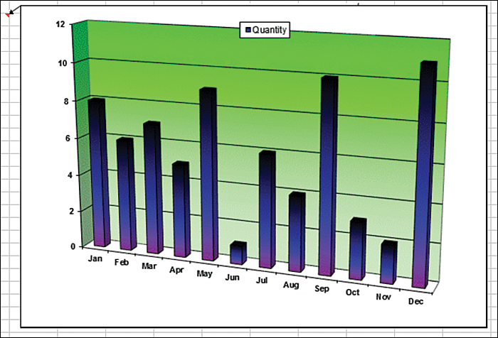
FIGURE 13-1 Place a chart in a cell note.
These are the steps to do this manually:
Create and save the picture image you want the note to display.
If you have not already done so, create the note and select the cell in which the note is located.
From the Review tab, select Notes, Edit Note or right-click the cell and select Edit Note.
Right-click the note border and select Format Comment.
Select the Colors And Lines tab and click the down arrow belonging to the Color field of the Fill section.
Select Fill Effects, select the Picture tab, and then click the Select Picture button.
Navigate to your desired image, select the image, and click OK twice.
The effect of having a “live chart” in a note can be achieved if, for example, the code is part of a SheetChange event when the chart’s source data is being changed. In addition, business charts are updated often, so you might want a macro to keep the note updated and to avoid repeating the same steps.
The following utility does just that—and you can use it by simply modifying the file pathname, chart name, destination sheet, cell, and size of the note shape, depending on the size of the chart:
Sub PlaceGraph()
Dim x As String, z As Range
Application.ScreenUpdating = False

'assign a temporary location to hold the image
x = "C:	empXWMJGraph.gif"

'assign the cell to hold the note
Set z = Worksheets("ChartInNote").Range("A3")

'delete any existing note in the cell
On Error Resume Next
z.Comment.Delete
On Error GoTo 0

'select and export the chart
ActiveSheet.ChartObjects("Chart 1").Activate
ActiveChart.Export x

'add a new note to the cell, set the size and insert the chart
With z.AddComment
    With .Shape
        .Height = 322
        .Width = 465
        .Fill.UserPicture x
    End With
End With

'delete the temporary image
Kill x

Range("A1").Activate
Application.ScreenUpdating = True

Set z = Nothing
End Sub
Tracking user changes
The Change event is a code solution posted often at Excel forums, primarily because it fills a void that formulas alone can’t manage (for example, inserting a date and time stamp when a user changes a specific range). The following utility takes advantage of the Change event in order to create a log file that tracks the cell address, new value, date, time, and username for changes made to column A of the sheet in which the code is placed.
This utility was submitted by our good friend Chris “Smitty” Smith of Redmond, Washington:
Private Sub Worksheet_Change(ByVal Target As Range)
'Code goes in the Worksheet specific module
Dim ws As Worksheet
Dim lr As Long
Dim rng As Range
'Set the Destination worksheet
Set ws = Sheets("Log Sheet")
'Get the first unused row on the Log sheet
lr = ws.Cells(Rows.Count, "A").End(xlUp).Row
'Set Target Range, i.e. Range("A1, B2, C3"), or Range("A1:B3")
Set rng = Target.Parent.Range("A:A")
'Only look at single cell changes
If Target.Count > 1 Then Exit Sub
'Only look at that range
If Intersect(Target, rng) Is Nothing Then Exit Sub
'Action if Condition(s) are met (do your thing here...)
'Put the Target cell's Address in Column A
ws.Cells(lr + 1, "A").Value = Target.Address
'Put the Target cell's value in Column B
ws.Cells(lr + 1, "B").Value = Target.Value
'Put the Date in Column C
ws.Cells(lr + 1, "C").Value = Date
'Put the Time in Column D
ws.Cells(lr + 1, "D").Value = Format(Now, "HH:MM:SS AM/PM")
'Put the Date in Column E
ws.Cells(lr + 1, "E").Value = Environ("UserName")
End Sub
Techniques for VBA pros
The utilities provided in the following sections amaze me. In the various message board communities on the Internet, VBA programmers are constantly coming up with new ways to do things faster and better. When someone posts some new code that obviously runs circles around the prior generally accepted best code, everyone benefits.
Creating an Excel state class module
This utility was submitted by Juan Pablo Gonzàlez Ruiz of Bogotà, Colombia. Juan Pablo is an Excel consultant who runs his photography business at www.juanpg.com.
The following class module is one of my favorites, and I use it in almost every project I create. Before Juan shared the module with me, I used to enter the eight lines of code to turn off and back on screen updating, events, alerts, and calculations. At the beginning of a sub, I would turn them off, and at the end I would turn them back on. That was quite a bit of typing. Now I just place the class module in a new workbook I create and call it as needed.
Insert a class module named CAppState and place the following code in it:
Private m_su As Boolean
Private m_ee As Boolean
Private m_da As Boolean
Private m_calc As Long
Private m_cursor As Long
Private m_except As StateEnum

Public Enum StateEnum
 None = 0
 ScreenUpdating = 1
 EnableEvents = 2
 DisplayAlerts = 4
 Calculation = 8
 Cursor = 16
End Enum

Public Sub SetState(Optional ByVal except As StateEnum = StateEnum.None)
m_except = except
With Application
    If Not m_except And StateEnum.ScreenUpdating Then
        .ScreenUpdating = False
    End If

    If Not m_except And StateEnum.EnableEvents Then
        .EnableEvents = False
    End If

    If Not m_except And StateEnum.DisplayAlerts Then
        .DisplayAlerts = False
    End If

    If Not m_except And StateEnum.Calculation Then
        .Calculation = xlCalculationManual
    End If

    If Not m_except And StateEnum.Cursor Then
        .Cursor = xlWait
    End If
End With
End Sub

Private Sub Class_Initialize()
With Application
     m_su = .ScreenUpdating
     m_ee = .EnableEvents
     m_da = .DisplayAlerts
     m_calc = .Calculation
     m_cursor = .Cursor
End With
End Sub

Private Sub Class_Terminate()
With Application
    If Not m_except And StateEnum.ScreenUpdating Then
        .ScreenUpdating = m_su
    End If

    If Not m_except And StateEnum.EnableEvents Then
        .EnableEvents = m_ee
    End If

    If Not m_except And StateEnum.DisplayAlerts Then
        .DisplayAlerts = m_da
    End If

    If Not m_except And StateEnum.Calculation Then
        .Calculation = m_calc
    End If

    If Not m_except And StateEnum.Cursor Then
        .Cursor = m_cursor
    End If
End With
End Sub
The following code is an example of calling the class module to turn off the various states, running your code, and then setting the states back:
Sub RunFasterCode
Dim appState As CAppState
Set appState = New CAppState
appState.SetState None
'run your code
'if you have any formulas that need to update, use
'Application.Calculate
'to force the workbook to calculate
Set appState = Nothing
End Sub
Drilling-down a pivot table
This is yet another utility submitted by Tom Urtis.
When you are double-clicking the data section, a pivot table’s default behavior is to insert a new worksheet and display that drill-down information on the new sheet. This utility serves as an option for convenience, to keep the drilled-down record sets on the same sheet as the pivot table (see Figure 13-2) so that you can delete them as you want.
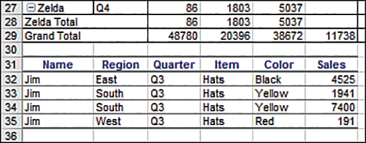
FIGURE 13-2 Show the drill-down record set on the same sheet as the pivot table.
To use this macro, double-click the data section or the totals section to create stacked drill-down record sets in the next available row of the sheet. To delete any drill-down record sets you have created, double-click anywhere in their respective current region.
Here’s the utility:
Private Sub Worksheet_BeforeDoubleClick(ByVal Target As Range, Cancel As Boolean)
Application.ScreenUpdating = False
Dim LPTR&

With ActiveSheet.PivotTables(1).DataBodyRange
    LPTR = .Rows.Count + .Row - 1
End With

Dim PTT As Integer
On Error Resume Next
PTT = Target.PivotCell.PivotCellType
If Err.Number = 1004 Then
    Err.Clear
    If Not IsEmpty(Target) Then
        If Target.Row > Range("A1").CurrentRegion.Rows.Count + 1 Then
            Cancel = True
            With Target.CurrentRegion
                .Resize(.Rows.Count + 1).EntireRow.Delete
            End With
        End If
    Else
        Cancel = True
    End If
Else
    CS = ActiveSheet.Name
End If
Application.ScreenUpdating = True
End Sub
Filtering an OLAP pivot table by a list of items
This utility was submitted by Jerry Sullivan of San Diego, California. Jerry is an operations manager for exp (www.exp.com), a building engineering consulting firm.
This procedure filters an OLAP pivot table to show items in a separate list, regardless of whether an item in that list has a matching record.
The code converts user-friendly items into MDX member references—for example, from “banana” to “[tblSales].[product_name].&[banana]"]”:
Sub FilterOLAP_PT()
'example showing call to function sOLAP_FilterByItemList

Dim pvt As PivotTable
Dim sErrMsg As String, sTemplate As String
Dim vItemsToBeVisible As Variant

On Error GoTo ErrProc
With Application
    .EnableCancelKey = xlErrorHandler
    .ScreenUpdating = False
    .DisplayStatusBar = False
    .EnableEvents = False
End With

'read filter items from worksheet table
vItemsToBeVisible = Application.Transpose( _
 wksPivots.ListObjects("tblVisibleItemsList").DataBodyRange.Value)

Set pvt = wksPivots.PivotTables("PivotTable1")
'call function
sErrMsg = sOLAP_FilterByItemList( _
     pvf:=pvt.PivotFields("[tblSales].[product_name].[product_name]"), _
     vItemsToBeVisible:=vItemsToBeVisible, _
     sItemPattern:="[tblSales].[product_name].&[ThisItem]")

ExitProc:
On Error Resume Next
With Application
     .EnableEvents = True
     .DisplayStatusBar = True
     .ScreenUpdating = True
End With
If Len(sErrMsg) > 0 Then MsgBox sErrMsg
Exit Sub

ErrProc:
sErrMsg = Err.Number & " - " & Err.Description
Resume ExitProc
End Sub

Private Function sOLAP_FilterByItemList(ByVal pvf As PivotField, _
 ByVal vItemsToBeVisible As Variant, _
 ByVal sItemPattern As String) As String

'filters an OLAP pivot table to display a list of items,
' where some of the items might not exist
'works by testing whether each pivotitem exists, then building an
' array of existing items to be used with the VisibleItemsList property

'Input Parameters:
'pvf - pivotfield object to be filtered
'vItemsToBeVisible - 1-D array of strings representing items to be visible
'sItemPattern - string that has MDX pattern of pivotItem reference
' where the text "ThisItem" will be replaced by each
' item in vItemsToBeVisible to make pivotItem references.
' e.g.: "[tblSales].[product_name].&[ThisItem]"

Dim lFilterItemCount As Long, lNdx As Long
Dim vFilterArray As Variant
Dim vSaveVisibleItemsList As Variant
Dim sReturnMsg As String, sPivotItemName As String

'store existing visible items
vSaveVisibleItemsList = pvf.VisibleItemsList

If Not (IsArray(vItemsToBeVisible)) Then _
 vItemsToBeVisible = Array(vItemsToBeVisible)
ReDim vFilterArray(1 To _
 UBound(vItemsToBeVisible) - LBound(vItemsToBeVisible) + 1)
pvf.Parent.ManualUpdate = True

'check if pivotitem exists then build array of items that exist
For lNdx = LBound(vItemsToBeVisible) To UBound(vItemsToBeVisible)
    'create MDX format pivotItem reference by substituting item into
    'pattern
    sPivotItemName = Replace(sItemPattern, "ThisItem", vItemsToBeVisible(lNdx))

    'attempt to make specified item the only visible item
    On Error Resume Next
    pvf.VisibleItemsList = Array(sPivotItemName)
    On Error GoTo 0

    'if item doesn't exist in field, this will be false
    If LCase$(sPivotItemName) = LCase$(pvf.VisibleItemsList(1)) Then
        lFilterItemCount = lFilterItemCount + 1
        vFilterArray(lFilterItemCount) = sPivotItemName
    End If
Next lNdx

'if at least one existing item found, filter pivot using array
If lFilterItemCount > 0 Then
    ReDim Preserve vFilterArray(1 To lFilterItemCount)
    pvf.VisibleItemsList = vFilterArray
Else
    sReturnMsg = "No matching items found."
    pvf.VisibleItemsList = vSaveVisibleItemsList
End If
pvf.Parent.ManualUpdate = False
sOLAP_FilterByItemList = sReturnMsg
End Function
Creating a custom sort order
This utility was submitted by Wei Jiang of Wuhan City, China.
By default, Excel enables you to sort lists numerically or alphabetically, but sometimes that is not what is needed. For example, a client might need each day’s sales data sorted by the default division order of belts, handbags, watches, wallets, and everything else. Although you can manually set up a custom series and sort using it, if you’re creating an automated workbook for other users, that might not be an option. This utility uses a custom sort order list to sort a range of data into default division order and then deletes the custom sort order, and Figure 13-3 shows the results:
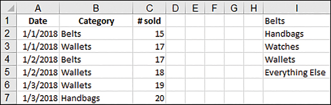
FIGURE 13-3 When you use the macro, the list in A:C is sorted first by date and then by the custom sort list in column I.
Sub CustomSort()
' add the custom list to Custom Lists
Application.AddCustomList ListArray:=Range("I1:I5")

' get the list number
nIndex = Application.GetCustomListNum(Range("I1:I5").Value)

' Now, we could sort a range with the custom list.
' Note, we should use nIndex + 1 as the custom list number here,
' for the first one is Normal order
Range("A2:C16").Sort Key1:=Range("B2"), Order1:=xlAscending, _
 Header:=xlNo, Orientation:=xlSortColumns, _
 OrderCustom:=nIndex + 1
Range("A2:C16").Sort Key1:=Range("A2"), Order1:=xlAscending, _
 Header:=xlNo, Orientation:=xlSortColumns

' At the end, we should remove this custom list...
Application.DeleteCustomList nIndex
End Sub
Creating a cell progress indicator
Here is another utility submitted by the prolific Tom Urtis.
I have to admit, the conditional formatting options in Excel, such as data bars, are fantastic. However, there still isn’t an option for a visual like the example shown in Figure 13-4. The following utility builds a progress indicator in column C, based on entries in columns A and B:
Private Sub Worksheet_Change(ByVal Target As Range)
If Target.Column > 2 Or Target.Cells.Count > 1 Then Exit Sub
If Application.IsNumber(Target.Value) = False Then
    Application.EnableEvents = False
    Application.Undo
    Application.EnableEvents = True
    MsgBox "Numbers only please."
    Exit Sub
End If
Select Case Target.Column
    Case 1
        If Target.Value > Target.Offset(0, 1).Value Then
            Application.EnableEvents = False
            Application.Undo
            Application.EnableEvents = True
            MsgBox "Value in column A may not be larger than value " & _
                "in column B."
            Exit Sub
        End If
    Case 2
        If Target.Value < Target.Offset(0, -1).Value Then
            Application.EnableEvents = False
            Application.Undo
            Application.EnableEvents = True
            MsgBox "Value in column B may not be smaller " & _
                "than value in column A."
            Exit Sub
        End If
End Select
Dim x As Long
x = Target.Row
Dim z As String
z = Range("B" & x).Value - Range("A" & x).Value
With Range("C" & x)
    .Formula = "=IF(RC[-1]<=RC[-2],REPT(""n"",RC[-1])&" & _
        "REPT(""n"",RC[-2]-RC[-1]),REPT(""n"",RC[-2])&" & _
        "REPT(""o"",RC[-1]-RC[-2]))"
    .Value = .Value
    .Font.Name = "Wingdings"
    .Font.ColorIndex = 1
    .Font.Size = 10
    If Len(Range("A" & x)) <> 0 Then
        .Characters(1, (.Characters.Count - z)).Font.ColorIndex = 3
        .Characters(1, (.Characters.Count - z)).Font.Size = 12
    End If
End With
End Sub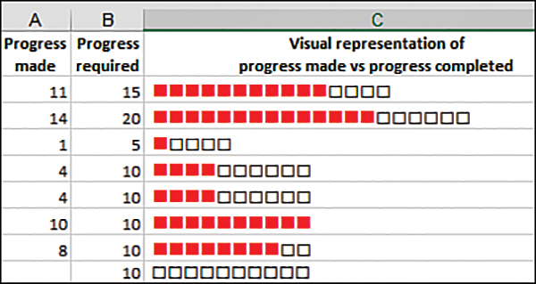
FIGURE 13-4 You can use indicators in cells to show progress.
Using a protected password box
This utility was submitted by Daniel Klann of Sydney, Australia. Daniel works mainly with VBA in Excel and Access but dabbles in all sorts of languages.
Using an input box for password protection has a major security flaw: The characters being entered are easily viewable. This program changes the characters to asterisks as they are entered—just like a real password field (see Figure 13-5). Note that the code that follows does not work in 64-bit Excel. Refer to Chapter 23, “The Windows Application Programming Interface (API),” for information on modifying the code for 64-bit Excel.
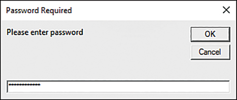
FIGURE 13-5 You can use an input box as a secure password field.
Here is the utility:
Private Declare Function CallNextHookEx Lib "user32" (ByVal hHook As Long, _
 ByVal ncode As Long, ByVal wParam As Long, lParam As Any) As Long

Private Declare Function GetModuleHandle Lib "kernel32" _
 Alias "GetModuleHandleA" (ByVal lpModuleName As String) As Long

Private Declare Function SetWindowsHookEx Lib "user32" Alias "SetWindowsHookExA" _
 (ByVal idHook As Long, ByVal lpfn As Long, _
 ByVal hmod As Long,ByVal dwThreadId As Long) As Long

Private Declare Function UnhookWindowsHookEx Lib "user32" _
 (ByVal hHook As Long) As Long

Private Declare Function SendDlgItemMessage Lib "user32" _
 Alias "SendDlgItemMessageA" (ByVal hDlg As Long, _
 ByVal nIDDlgItem As Long, ByVal wMsg As Long, _
 ByVal wParam As Long, ByVal lParam As Long) As Long

Private Declare Function GetClassName Lib "user32" _
 Alias "GetClassNameA" (ByVal hwnd As Long, _
 ByVal lpClassName As String, ByVal nMaxCount As Long) As Long

Private Declare Function GetCurrentThreadId Lib "kernel32" () As Long

'Constants to be used in our API functions
Private Const EM_SETPASSWORDCHAR = &HCC
Private Const WH_CBT = 5
Private Const HCBT_ACTIVATE = 5
Private Const HC_ACTION = 0

Private hHook As Long

Public Function NewProc(ByVal lngCode As Long, _
 ByVal wParam As Long, ByVal lParam As Long) As Long
Dim RetVal
Dim strClassName As String, lngBuffer As Long

If lngCode < HC_ACTION Then
    NewProc = CallNextHookEx(hHook, lngCode, wParam, lParam)
    Exit Function
End If

strClassName = String$(256, " ")
lngBuffer = 255

If lngCode = HCBT_ACTIVATE Then 'A window has been activated

    RetVal = GetClassName(wParam, strClassName, lngBuffer)

    'Check for class name of the Inputbox
    If Left$(strClassName, RetVal) = "#32770" Then
        'Change the edit control to display the password character *.
        'You can change the Asc("*") as you please.
        SendDlgItemMessage wParam, &H1324, EM_SETPASSWORDCHAR, Asc("*"), &H0
    End If

End If

'This line will ensure that any other hooks that may be in place are
'called correctly.
CallNextHookEx hHook, lngCode, wParam, lParam
End Function

Public Function InputBoxDK(Prompt, Optional Title, _
 Optional Default, Optional XPos, _
 Optional YPos, Optional HelpFile, Optional Context) As String
 Dim lngModHwnd As Long, lngThreadID As Long

 lngThreadID = GetCurrentThreadId
 lngModHwnd = GetModuleHandle(vbNullString)

 hHook = SetWindowsHookEx(WH_CBT, AddressOf NewProc, lngModHwnd, lngThreadID)
 On Error Resume Next
 InputBoxDK = InputBox(Prompt, Title, Default, XPos, YPos, HelpFile, Context)
 UnhookWindowsHookEx hHook
End Function

Sub PasswordBox()
If InputBoxDK("Please enter password", "Password Required") <> "password" Then
    MsgBox "Sorry, that was not a correct password."
Else
     MsgBox "Correct Password! Come on in."
End If
End Sub
Selecting with SpecialCells
This utility was submitted by Ivan F. Moala of Auckland, New Zealand.
Typically, when you want to find certain values, text, or formulas in a range, the range is selected, and each cell is tested. The following utility shows how you can use SpecialCells to select only the desired cells. Having fewer cells to check speeds up your code.
The following code ran in the blink of an eye on my machine. However, the version that checked each cell in the range (A1:Z20000) took 14 seconds—an eternity in the automation world!
Sub SpecialRange()
Dim TheRange As Range
Dim oCell As Range

Set TheRange = Range("A1:Z20000").SpecialCells(xlCellTypeConstants, xlTextValues)

For Each oCell In TheRange
    If oCell.Text = "Your Text" Then
        MsgBox oCell.Address
        MsgBox TheRange.Cells.Count
    End If
Next oCell
End Sub
Resetting a table’s format
Here’s another utility submitted by Zack Barresse.
Tables are great tools to use, but they’re not perfect. One issue you’ll eventually run into is a table’s formatting acting up. For example, formatting might suddenly no longer be applied to new rows. The following procedure resets a table’s format so it functions properly:
Sub ResetFormat(ByVal Table As ListObject, _
 Optional ByVal RetainNumberFormats As Boolean = True)
Dim Formats() As Variant
Dim ColumnStep As Long

If Table.Parent.ProtectContents = True Then
    MsgBox "The worksheet is protected.", vbExclamation, "Whoops!"
    Exit Sub
End If

If RetainNumberFormats Then
    ReDim Formats(Table.ListColumns.Count - 1)
    For ColumnStep = 1 To Table.ListColumns.Count
        On Error Resume Next
        Formats(ColumnStep - 1) = Table.ListColumns(ColumnStep). _
            DataBodyRange.NumberFormat
        On Error GoTo 0
        If IsEmpty(Formats(ColumnStep - 1)) Then
             Formats(ColumnStep - 1) = "General"
        End If
    Next ColumnStep
End If

Table.Range.Style = "Normal"

If RetainNumberFormats Then
    For ColumnStep = 1 To Table.ListColumns.Count
        On Error Resume Next
        Table.ListColumns(ColumnStep).DataBodyRange.NumberFormat = _
            Formats(ColumnStep - 1)
        On Error GoTo 0
        If Err.Number <> 0 Then
            Table.ListColumns(ColumnStep).DataBodyRange.NumberFormat = _
                 "General"
            Err.Clear
        End If
    Next ColumnStep
End If
End Sub
Using VBA Extensibility to add code to new workbooks
Say that you have a macro that moves data to a new workbook for the regional managers. What if you need to also copy macros to the new workbook? You can use VBA Extensibility to import modules to a workbook or to actually write lines of code to the workbook.
To use any of the following examples, you must trust access to VBA by going to the Developer tab, choosing Macro Security, and checking Trust Access To The VBA Project Object Model.
The easiest way to use VBA Extensibility is to export a complete module or userform from the current project and import it to the new workbook. Perhaps you have an application with thousands of lines of code, and you want to create a new workbook with data for the regional manager and give her three macros to enable custom formatting and printing. Place all of these macros in a module called modToRegion. Macros in this module also call the frmRegion userform. The following code transfers this code from the current workbook to the new workbook:
Sub MoveDataAndMacro()
Dim WSD as worksheet
Set WSD = Worksheets("Report")
' Copy Report to a new workbook
WSD.Copy
' The active workbook is now the new workbook
' Delete any old copy of the module from C
On Error Resume Next
' Delete any stray copies from hard drive
Kill ("C:	empModToRegion.bas")
Kill ("C:	empfrmRegion.frm")
On Error GoTo 0
' Export module & form from this workbook
ThisWorkbook.VBProject.VBComponents("ModToRegion").Export _
 ("C:	empModToRegion.bas")
ThisWorkbook.VBProject.VBComponents("frmRegion").Export _
 ("C:	empfrmRegion. frm")
' Import to new workbook
ActiveWorkbook.VBProject.VBComponents.Import ("C:	empModToRegion.bas")
ActiveWorkbook.VBProject.VBComponents.Import ("C:	empfrmRegion.frm")
On Error Resume Next
Kill ("C:	empModToRegion.bas")
Kill ("C:	empfrmRegion.bas")
On Error GoTo 0
End Sub
This method works if you need to move modules or userforms to a new workbook. However, what if you need to write some code to the Workbook_Open macro in the ThisWorkbook module? There are two tools to use. The Lines method enables you to return a particular set of code lines from a given module. The InsertLines method enables you to insert code lines to a new module.
![]() Note
Note
With each call to InsertLines, you must insert a complete macro. Excel attempts to compile the code after each call to InsertLines. If you insert lines that do not completely compile, Excel might crash with a general protection fault (GPF).
Sub MoveDataAndMacro()
Dim WSD as worksheet
Dim WBN as Workbook
Dim WBCodeMod1 As Object, WBCodeMod2 As Object
Set WSD = Worksheets("Report")
' Copy Report to a new workbook
WSD.Copy
' The active workbook is now the new workbook
Set WBN = ActiveWorkbook
' Copy the Workbook level Event handlers
Set WBCodeMod1 = ThisWorkbook.VBProject.VBComponents("ThisWorkbook") _
 .CodeModule
Set WBCodeMod2 = WBN.VBProject.VBComponents("ThisWorkbook").CodeModule
WBCodeMod2.InsertLines 1, WBCodeMod1.Lines(1, WBCodeMod1.countoflines)
End Sub
Converting a fixed-width report to a data set
This is my own submission. I’ve been writing a lot of cleaning programs for clients lately and realized this was a good example of using a class, collection, and array to accomplish the task. Also included is a function for checking if a record exists in a collection.
Imagine you request customer information and receive the data in a report format, as shown in Figure 13-6. Each customer record consists of two rows, some information is missing, and there are duplicate records.
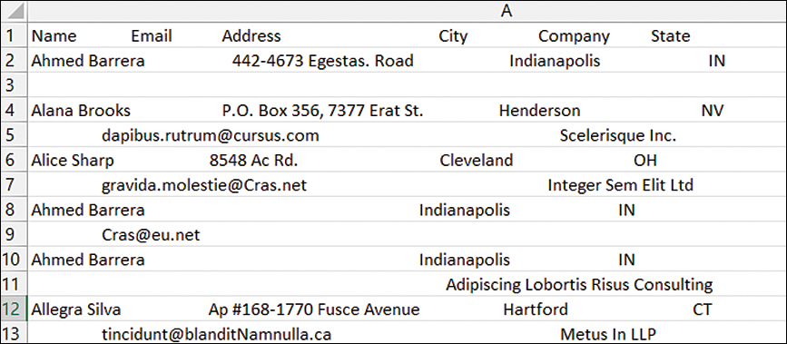
FIGURE 13-6 Extracting data from a report may seem near impossible, but with a little ingenuity and code, it can be done.
The class is used to clean and organize the customer data. The collection is used to ensure I only have unique records, but also allows me to merge duplicate records. Finally, the array is sized for just the unique records and quickly places the results on the sheet.
Place the following in a class module named clsRecord:
Private m_UserName As String
Private m_StreetAddress As String
Private m_City As String
Private m_State As String
Private m_Company As String
Private m_Email As String

Public Property Let currentRecord(RHS As String)
'the 2 row record is broken up when it's passed in
CleanRecord RHS
End Property
Public Property Get UserName() As String
UserName = m_UserName
End Property
Public Property Get StreetAddress() As String
StreetAddress = m_StreetAddress
End Property
Public Property Get City() As String
City = m_City
End Property
Public Property Get State() As String
State = m_State
End Property
Public Property Get Company() As String
Company = m_Company
End Property
Public Property Get Email() As String
Email = m_Email
End Property

Private Sub CleanRecord(ByVal curRecord As String)

If Len(Trim(curRecord)) = 0 Then Exit Sub 'no data

'if some data is missing, it can throw off the Mid statements
'so we use On Error Resume Next to keep the code moving
On Error Resume Next
If Trim(Left(curRecord, 1)) <> "" Then
   'if there's data in position 1, we have a 1st row record
   If m_UserName = "" Then m_UserName = Trim(Left(curRecord, 34))
   If m_StreetAddress = "" Then m_StreetAddress = Trim(Mid(curRecord, 35, 45))
   If m_City = "" Then m_City = Trim(Mid(curRecord, 80, 37))
   If m_State = "" Then m_State = _
         Trim(Mid(curRecord, 117, Len(curRecord) - 116))
Else
   'else, it's a 2nd row record
   If m_Email = "" Then m_Email = Trim(Mid(curRecord, 18, 83))
   If m_Company = "" Then m_Company = _
      Trim(Mid(curRecord, 101, Len(curRecord) - 100))
End If

On Error GoTo 0
End Sub
Place the following in a standard module:
Enum Report
   UserName = 1
   StreetAddress
   City
   State
   Email
   Company
End Enum

Sub CleanReport()
Dim cRecord As clsRecord
Dim AllRecords As Collection: Set AllRecords = New Collection
Dim rawData, FinalData
Dim errMessage As String, UserNameKey As String
Dim eaRecord As Long

rawData = Worksheets("Data").Range("A1:A203")
On Error GoTo errHandler
For eaRecord = 2 To UBound(rawData) Step 2
   UserNameKey = Trim(Left(rawData(eaRecord, 1), 34))
   'check if we already have the record in the collection
   If GetFromCollection(UserNameKey, AllRecords, cRecord, True, errMessage) Then
      'delete the original
      AllRecords.Remove UserNameKey
   Else
      'initialize a new Record
      Set cRecord = New clsRecord
   End If
   'send current record set to class for cleaning
   cRecord.currentRecord = rawData(eaRecord, 1)
   cRecord.currentRecord = rawData(eaRecord + 1, 1)

   'save the record to the collection
   AllRecords.Add cRecord, CStr(UserNameKey)
Next eaRecord

'place final records into array
ReDim FinalData(1 To AllRecords.Count, 1 To 6)
For eaRecord = 1 To AllRecords.Count
   Set cRecord = AllRecords(eaRecord)
   FinalData(eaRecord, Report.UserName) = cRecord.UserName
   FinalData(eaRecord, Report.StreetAddress) = cRecord.StreetAddress
   FinalData(eaRecord, Report.City) = cRecord.City
   FinalData(eaRecord, Report.State) = cRecord.State
   FinalData(eaRecord, Report.Email) = cRecord.Email
   FinalData(eaRecord, Report.Company) = cRecord.Company
Next eaRecord

With Worksheets("Report")
   .Range("A1").Resize(, 6).Value = _
         Array("Name", "Address", "City", "State", "Email", "Company")
   .Range("A2").Resize(UBound(FinalData), UBound(FinalData, 2)).Value = FinalData
End With

errHandler:
If Err.Number <> 0 Then
   MsgBox Err.Number & ": " & Err.Description
End If

Set AllRecords = Nothing
Set cRecord = Nothing
End Sub

Function GetFromCollection(ByVal KeyName As String, _
   ByVal CollectionToSearch As Collection, ByRef ReturnedValue As Variant, _
   ByVal ReturnObject As Boolean, ByRef errMessage As String) As Boolean
GetFromCollection = True
On Error Resume Next
If ReturnObject Then
    Set ReturnedValue = CollectionToSearch(KeyName)
Else
    ReturnedValue = CollectionToSearch(KeyName)
End If
If Err.Number <> 0 Then GetFromCollection = False
On Error GoTo 0
End Function
Next steps
The utilities in this chapter aren’t Excel’s only source of programming power. User-defined functions (UDFs) enable you to create complex custom formulas to cover what Excel’s functions don’t. In Chapter 14, “Sample user-defined functions,” you’ll find out how to create and share your own functions.