
Chapter 7
Understanding Functions
Excel is used on 750 million desktops around the world. People in all career types use Excel, as do many home users who take advantage of Excel’s powerful features to track their finances, investments, and more. Part of Excel’s versatility is its wide range of built-in functions.
Excel 2019 offers 474 built-in calculation functions. This number grows with each new release. Excel 2019 debuts six new functions: CONCAT, IFS, MAXIFS, MINIFS, SWITCH, and TEXTJOIN. By the end of 2018, Office 365 introduced SORT, SORTBY, FILTER, UNIQUE, and SINGLE, bringing the function count to 479.
Working with Functions
To use functions successfully in a worksheet, you need to follow the function syntax. Keep in mind that a formula that makes use of a function needs to start with an equal sign. You type the function name, an opening parenthesis, function arguments (separated by commas), and the closing parenthesis.
The general syntax of a function looks like this:
=FunctionName(Argument1,Argument2,Argument3)
Parentheses are needed with every function, including functions that require no arguments. For example, these functions still require the parentheses:
=NOW()
=DATE()
=TODAY()
=PI()
The arguments for a function should be entered in the correct order, as specified in this book or Excel Help. For example, the PMT() function expects the arguments to have the interest rate first, followed by the number of periods, followed by the present value. If you attempt to send the arguments in the wrong order, Excel happily calculates the wrong result.
In many cases, you can enter arguments as numbers or as cell references. For example, all these formulas are valid:
=SUM(1,2,3^2,4/5,6*7)
=SUM(A1:A9,C1,D2,Sheet2!E3:M10)
=SUM(A1:A9,100,200,B3*5)
Note
Chapters 8, “Using Everyday Functions: Math, Date and Time, and Text Functions,” and 9, “Using Powerful Functions: Logical, Lookup, Web, and Database Functions,” cover many interesting functions. This chapter covers a number of the most commonly used functions.
Note
Excel functions can return some errors. This happens most frequently when one of the arguments passed to the function is outside the range of what the function expects. When you receive a #NUM!, #VALUE!, or #N/A error, you should look in Excel Help for the function. The Remarks section usually indicates exactly what problems can cause each type of error.
The Formulas Tab in Excel 2019
One way to find functions in Excel 2019 is on the Formulas tab. This tab offers the Insert Function, AutoSum, Recently Used, Financial, Logical, Text, Date & Time, Lookup & Reference, Math & Trig, and More Functions icons.
As shown in Figure 7.1, when you click the More Functions icon, a drop-down menu with six additional function groups—Statistical, Engineering, Cube, Information, Compatibility, and Web—appears.

The Formulas tab is designed to make it easier to find the right function. You select an icon from the ribbon, and an alphabetical list of functions in that group appears. If you hover your mouse over a function in the list, Excel displays a description of what the function does, as shown in Figure 7.2.
Finding the Function You Need
The inherent problem with the Formulas tab is that you often have to guess where your desired function might be hiding. The function categories have been established in Excel for a decade, and in some cases, functions are tucked away in strange places.
For example, the SUM() function is a Math & Trig function. This makes sense because adding numbers is clearly a mathematical process. However, the AVERAGE() function is not available in the Math & Trig icon. (It is under More Functions, Statistical.) The COUNT() function could be math, reference, or information, but it is found under More Functions, Statistical.
By dividing the list of functions into categories, Microsoft has made it rather difficult to find certain functions. Fortunately, as described in the following sections, you can use some tricks to make this process simpler.
Using Tab to AutoComplete Functions
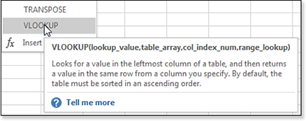
One feature in Excel 2019 is Formula AutoComplete. Sometimes you might remember part of the function name but not the name. For example, if you type =LOOK, Excel will offer LOOKUP, HLOOKUP, and VLOOKUP. Rather than trying to figure out which category on the Formulas tab contains your function, you can just start typing =LOOK into a cell. Excel displays a pop-up window with all the functions that contain LOOK, as shown in Figure 7.3. This feature has been changed since Excel 2016. Previously, typing =LOO would not have returned VLOOKUP or HLOOKUP because the AutoComplete only matched from the beginning of a word.

=LOOK to display a list of the Lookup functions.To accept a function name from the list, you can either double-click the function name or select the name and press Tab.
Using the Insert Function Dialog Box to Find Functions
A large Insert Function icon appears on the Formula tab of the ribbon. This command is repeated at the bottom of every function category. These 14 new entry points for Insert Function were added in Excel 2007, but it is easier to use the fx icon located to the left of the formula bar. Click the fx, and the Insert Function dialog box appears.
Use the Search for a Function box to locate the function. For example, if you typed loan payment and then clicked Go, Excel would suggest PMT (the correct function) as well as PPMT, ISPMT, RATE, and others.
When you choose a function in the Insert Function dialog box, the dialog box displays the syntax for the function, as well as a one-sentence description of the function, as shown in Figure 7.4. If you need more details, you can click the Help On This Function hyperlink in the lower-left corner of the Insert Function dialog box.

Getting Help with Excel Functions
Every Excel function has three levels of help:
On-grid ToolTip
Function Arguments dialog box
Excel Help
Tip
If you type
=FunctionName(in a cell, you can press Ctrl+A anytime after the opening parenthesis to display the Function Arguments dialog box.
The following sections discuss these levels of help. However, you are sure to find the Function Arguments dialog box to be one of the best ways of getting help.
Using On-Grid ToolTips
In any cell, you can type an equal sign, a function name, and the opening parenthesis. Excel displays a ToolTip that shows the expected arguments. In many cases, this ToolTip is enough to guide you through the function. For example, I can usually remember that the function for figuring out a car loan payment is =PMT(), but I can never remember the order of the arguments. The ToolTip, as shown in Figure 7.5, is enough to remind me that rate comes first, followed by the number of periods, and then the principal amount or present value. Any function arguments displayed in square brackets are optional, so in the example shown in Figure 7.5, you know that you may not have to enter anything for fv or type.
![This figure shows the Excel grid after typing =PMT(. A tooltip shows PMT(rate, nper, pv, [fv], [type]). If you click PMT, you get help for that argument. Click any argument name to jump to that portion of the formula.](http://images-20200215.ebookreading.net/7/3/3/9781509306015/9781509306015__microsoft-excel-2019__9781509306015__graphics__07fig05.jpg)
As you type each comma in the function, the next argument in the ToolTip lights up in boldface. This way, you always know which argument you are entering.
Tip
By the way, you can click the formula ToolTip and drag it to a new location on the worksheet. This can be useful if the ToolTip is covering cells that you need to click when building the function.
If you click the function name in the ToolTip, Excel opens Help for that function.
Using the Function Arguments Dialog Box
When you access a function through the Function Wizard or a drop-down menu, Excel displays the Function Arguments dialog box. This dialog box is one of the best features in Excel. If you’ve started to type the function and typed the opening parenthesis, then pressing Ctrl+A or clicking the fx icon to the left of the formula bar displays the Function Arguments dialog box.
As shown in Figure 7.6, the Function Arguments dialog box has many elements:
The one-sentence description of the function appears in the center of the dialog box.
As you tab into the text box for each argument, the description of the argument is shown in the dialog box. This description guides you as to what Excel is expecting. For example, in the dialog box shown in Figure 7.6, Excel reminds you that the interest rate needs to be divided by four for quarterly payments. This reminds you to divide the rate in cell B3 by 12 for monthly payments.
To the right of each argument in the dialog box is a reference button. You can click this button to collapse the dialog box so you can point to the cells for that argument.
To the right of each text box is a label that shows the result of the entry for that argument.
Any arguments in bold are required. Arguments not in bold are optional.
After you enter the required arguments, the dialog box shows the preliminary result of the formula. This is on the right side, just below the last argument text box. It appears again in the lower-left corner, just above the Help On This Function hyperlink.
A Help On This Function hyperlink to the Help topic for the function appears in the lower-left corner of the dialog box.

Figure 7.6 The Function Arguments dialog box helps you build a function, one step at a time. Troubleshooting
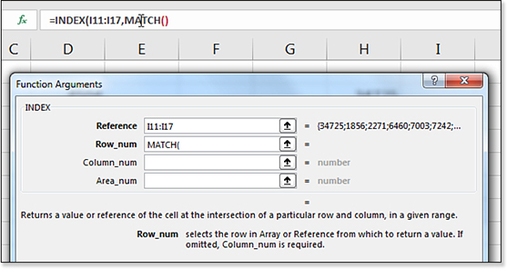
How can you use the Function Arguments dialog when you have a nested function? For example, if you are using MATCH inside of INDEX.
Start by typing the =INDEX( function and press Ctrl+A to display the Function Arguments.
In the second Row_Num box of the Function Arguments dialog box, type MATCH(.
Using your mouse, reach up to the formula bar and click inside of the word MATCH. The Function Arguments dialog will switch to display the arguments for MATCH. When you complete the MATCH function and you want to return to the INDEX version of the Function Arguments dialog box, use the mouse to click on INDEX in the Formula Bar.
Using Excel Help
The Excel Help topics for the functions are incredibly complete. Each function’s Help topic includes the following sections:
The function syntax appears at the top of the topic. This includes a description of each function that might be more complete than the description in the Function Arguments dialog box.
The Remarks section helps troubleshoot possible problems with the function. It discusses specific limits for each argument and describes the meaning of each possible error that could be returned from the function.
Each function has an example section composed of an embedded Excel Web App worksheet. You can click the XL icon in the footer of the example to download the example to your computer.
The See Also section at the bottom of a Help topic enables you to discover related functions. The logical groupings suggested by See Also are far more useful than the category groupings in the Formulas tab.
Using AutoSum
Microsoft realizes that the most common function is the SUM() function. It is so popular that Excel provides one-click access to the AutoSum feature.
The AutoSum icon is the large Greek letter sigma that is the second icon on the Formulas tab or a small icon on the right side of the Home tab. You can click this icon to use AutoSum, or you can use the drop-down menu at the bottom of the icon to access AutoSum versions of Average, Count Numbers, Max, and Min, as shown in Figure 7.7.

Tip
Pressing Alt+= is equivalent to clicking the AutoSum icon.
When you click the AutoSum button, Excel seeks to add up the numbers that are above or to the left of the current cell. In general, when you click the AutoSum icon, Excel guesses which cells you are trying to sum. Excel automatically types the SUM() formula. You should review Excel’s guess to make sure that Excel chose the correct range to sum. In Figure 7.8, for example, Excel correctly guesses that you want to sum the column of quantities above the cell.

Potential Problems with AutoSum
Although you should always check the range proposed by the AutoSum feature, in some cases you should be especially wary. If the headings above the data are numeric, for example, this will fool AutoSum. In Figure 7.9, the 2019 heading in B1 is numeric. This causes Excel to include the heading incorrectly in the total for column B.

When Excel proposes the wrong range for a sum, use your mouse to highlight the correct range before pressing Enter.
Excel avoids including other SUM() functions in an AutoSum range. If a range contains a SUM() function that references other cells, Excel prematurely stops just before the SUM() function. This problem happens only when the SUM() function references other cells. If the cell contained =7000+1878 or =H3+H4 or =SUM(7000,1878), AutoSum would include the cell.
Excel prefers to sum a column of numbers instead of a row of numbers. Figure 7.10 shows a strange anomaly. If you place the cell pointer in cell F2 and click AutoSum, Excel correctly guesses that you want to total B2:E2. Cell F3 works fine. However, when you get to cell F4, Excel has a choice. There are two numbers above F4 and four numbers to the left of F4. Because there are two numbers directly above, Excel tries to total those two numbers. This problem seems to happen only in the third row of the data set. After that, Excel sees that the three cells above are all summing across the rows, and AutoSum works perfectly in F5:F10.

Special Tricks with AutoSum
There is an amazing trick you can use with AutoSum. If you select a range of cells before clicking the AutoSum button, Excel does a much better job of predicting what to sum.
In Figure 7.10, for example, you could select B11:E11 before clicking the AutoSum button, and Excel would know to sum each column. Be careful, though, because Excel does not preview its guess before entering the formula. You should always check a formula after using AutoSum to make sure the correct range was selected.
If your selection contains a mix of blank cells and nonblank cells, Excel adds the AutoSum to only the blank cells. In Figure 7.11, for example, you select the range B2:F11 before clicking the AutoSum button.

After you click the AutoSum button, Excel correctly fills in totals for all the rows and columns, as shown in Figure 7.12.

SUM() formulas with one click.Using AutoAverage or AutoCount
The AutoSum button includes a drop-down menu arrow with choices for Average, Count, Max, and Min. If you find yourself frequently using the choices in this drop-down menu, you can add an icon to the Quick Access Toolbar that will AutoAverage, AutoCount, and so on. Open the AutoSum drop-down menu. Right-click Average and choose Add To Quick Access Toolbar to have one-click access to an icon that works similar to AutoSum but uses the AVERAGE calculation instead (see Figure 7.13).

Caution
Microsoft uses the same green circle icon to represent Average, Count, Max, and Min. If you are going to add all four icons to the Quick Access Toolbar, add them in alphabetical order to help you remember the sequence in which they appear.
Function Reference Chapters
Chapters 8 and 9 provide a fairly comprehensive reference for the common functions in Excel. Chapter 10, “Other Functions,” provides a reference of the remaining functions.
Function coverage is broken out as follows:
Chapter 8 describes functions that many people encounter in their everyday lives: some of the math functions, date functions, and text functions.
Chapter 9 describes functions that are a bit more difficult, but that should be a part of your everyday arsenal. These include a series of functions for making decisions in a formula. They include the
IFfunction and are known collectively as the logical functions. Chapter 9 also describes the information, lookup, and database functions.Chapter 10 provides a reference for financial, statistical, trigonometry, and engineering functions.