
Chapter 3. Basic SQL
As mentioned in Chapter 2, Dr. Edgar F. Codd conceived the relational database model in 1969 and its normal forms in the early 70’s. In IBM laboratories, in San Jose, a major research project started in the early 1970s called System/R, intending to prove the viability of the relational model. At the same time, in 1974, Dr. Donald Chamberlin and his colleagues were also working to define a database language. They developed Structured English Query Language (SEQUEL), which allowed users to query a relational database using clearly defined English-style sentences which later on was renamed to SQL (Structured Query Language or SQL Query Language) for legal reasons.
The first database management systems based on SQL became available commercially by the end of the 70s. And with the growing activity surrounding the development of database languages, the idea of standardization emerged to simplify the things. SQL was elected for standardization. Both the American ANSI and the international ISO took part in the standardization and, in 1986, the first SQL standard was approved. After that, several versions existed. It is common to refer the SQL standards as “SQL:1999”, “SQL:2003”, “SQL:2008”, and “SQL:2011” and they refer to the versions of the standard released in the corresponding years, with the last being the most recent version. We will use the phrase “the SQL standard” or “standard SQL” to mean the current version of the SQL Standard at any time.
MySQL extends the standard SQL providing extra features. For example, MySQL implements the STRAIGHT_JOIN which is not recognized by other RDBMS’s like Postgres.
This chapter introduces the basics of MySQL’s implementation of SQL which is often called as CRUD operations. The acronym CRUD refers to CREATE, READ, UPDATE and DELETE operations. We will show you how to read data from a database with the SELECT statement, and how to choose what data is returned and the order it is displayed in. We also show you the basics of modifying your databases with the INSERT statement to add data, UPDATE to change, and DELETE to remove it. We also explain how to use the nonstandard SHOW TABLES and SHOW COLUMNS statements to explore your database.
Using the Sakila Database
In Chapter 2, we showed you the principles of how to build a database diagram using the ER model. We also introduced the steps you take to convert an ER model to a format that makes sense for constructing a relational database. In this section, for you to start get familiar with different database relational models, we will show you the structure of the MySQL Sakila database. We are not going to explain the SQL statements used to create the database at this moment; that’s the subject of Chapter 4.
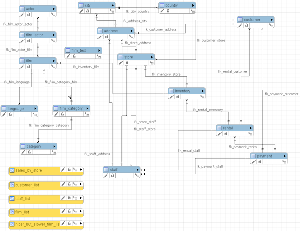
Figure 3-1. The ER diagram of the sakila database
To begin exploring the sakila database, you can download the data from the official repository.
The sakila-schema.sql file contains all the CREATE statements required to create the structure of the Sakila database including tables, views, stored procedures, and triggers.
The sakila-data.sql file contains the INSERT statements required to populate the structure created by the sakila-schema.sql file, along with definitions for triggers that must be created after the initial data load.
The sakila.mwb file is a MySQL Workbench data model that you can open within MySQL Workbench to examine the database structure.
To install the Sakila sample database, follow these steps:
-
Extract the installation archive to a temporary location such as C: emp or /tmp/. When you unpack the archive, it creates a directory named
sakila-dbthat contains thesakila-schema.sqlandsakila-data.sqlfiles.
Connect to the MySQL server using the mysql command-line client with the following command:
shell> mysql -u root -p
Enter your password when prompted. A non-root account can be used, provided that the account has privileges to create new databases.
Execute the sakila-schema.sql script to create the database structure, and execute the sakila-data.sql script to populate the database structure, by using the following commands:
mysql> SOURCE C:/temp/sakila-db/sakila-schema.sql;
mysql> SOURCE C:/temp/sakila-db/sakila-data.sql;
Replace the paths to the sakila-schema.sql and sakila-data.sql files with the actual paths on your system.
Now let’s explore the sakila database. To choose the sakila database as your current database, type the following:
mysql> USE sakila;
Database changed
mysql>
You can check that this is the active database by typing in the SELECT DATABASE( ); command:
mysql> SELECT DATABASE();------------| DATABASE() |------------| sakila |------------1 row in set (0.00 sec)
Now, let’s explore what tables make up the sakila database using the SHOW TABLES statement:
----------------------------| Tables_in_sakila |----------------------------| actor | | actor_info | | address | | category | | city | | country | | customer | | customer_list | | film | | film_actor | | film_category | | film_list | | film_text | | inventory | | language | | nicer_but_slower_film_list | | payment | | rental | | sales_by_film_category | | sales_by_store | | staff | | staff_list | | store |----------------------------23 rows in set (0.00 sec)
So far, there have been no surprises. Let’s find out more about each of the tables that make up the sakila database. First, let’s use the SHOW COLUMNS statement to explore the actor table:
mysql> SHOW COLUMNS FROM actor;-------------------------------------------------------------------------------------------------------------+ | Field | Type | Null | Key | Default | Extra |-------------------------------------------------------------------------------------------------------------+ | actor_id | smallint unsigned | NO | PRI | NULL | auto_increment | | first_name | varchar(45) | NO | | NULL | | | last_name | varchar(45) | NO | MUL | NULL | | | last_update | timestamp | NO | | CURRENT_TIMESTAMP | DEFAULT_GENERATED on update CURRENT_TIMESTAMP |-------------------------------------------------------------------------------------------------------------+ 4 rows in set (0.01 sec)
The DESCRIBE keyword is identical to SHOW COLUMNS FROM, and can be abbreviated to just DESC, so we can write the previous query as follows:
mysql> DESC actor;-------------------------------------------------------------------------------------------------------------+ | Field | Type | Null | Key | Default | Extra |-------------------------------------------------------------------------------------------------------------+ | actor_id | smallint unsigned | NO | PRI | NULL | auto_increment | | first_name | varchar(45) | NO | | NULL | | | last_name | varchar(45) | NO | MUL | NULL | | | last_update | timestamp | NO | | CURRENT_TIMESTAMP | DEFAULT_GENERATED on update CURRENT_TIMESTAMP |-------------------------------------------------------------------------------------------------------------+ 4 rows in set (0.00 sec)
Let’s examine the table structure more closely. The actor table contains four columns, actor_id, first_name, last_name and last_update. Another information we can extract from the output are the types of the columns — a smallint for actor_id, a varchar(45) for first_name and last_name and a timestamp for last_update. None of the columns accept to be NULL (empty), actor_id is the Primary Key and last_name is the first column of a nonunique index. Don’t worry about the details; all that’s important right now are the column names which will be used for the SQL commands.
Let’s explore another table. Here are the SHOW COLUMNS statements you need to type:
mysql> DESC city;-------------------------------------------------------------------------------------------------------------+ | Field | Type | Null | Key | Default | Extra |-------------------------------------------------------------------------------------------------------------+ | city_id | smallint unsigned | NO | PRI | NULL | auto_increment | | city | varchar(50) | NO | | NULL | | | country_id | smallint unsigned | NO | MUL | NULL | | | last_update | timestamp | NO | | CURRENT_TIMESTAMP | DEFAULT_GENERATED on update CURRENT_TIMESTAMP |-------------------------------------------------------------------------------------------------------------+ 4 rows in set (0.01 sec)
Again, what’s important is getting familiar with the columns in each table, as we’ll make use of these frequently later when we’re learning about querying.
In the next section, we show you how to explore the data that’s stored in the sakila database and its tables.
The SELECT Statement and Basic Querying Techniques
Up to this point, you’ve learned how to install and configure MySQL, and how to use the MySQL command line. Now that you understand the ER model, you’re ready to start exploring its data and to learn the SQL language that’s used by all MySQL clients. In this section, we introduce the most commonly used SQL keyword: the SELECT keyword. We also explain some basic elements of style and syntax, and the features of the WHERE clause, Boolean operators, and sorting (much of this also applies to our later discussions of INSERT, UPDATE, and DELETE). This isn’t the end of our discussion of SELECT; you’ll find more in [Link to Come], where we show you how to use its advanced features.
Single Table SELECTs
The most basic form of SELECT reads the data in all rows and columns from a table. Connect to MySQL using the command line and choose the sakila database:
mysql> use sakila;
Database changed
Let’s retrieve all of the data in the language table:
mysql(sakila)> SELECT * FROM language;--------------------------------------------| language_id | name | last_update |--------------------------------------------| 1 | English | 2006-02-15 05:02:19 | | 2 | Italian | 2006-02-15 05:02:19 | | 3 | Japanese | 2006-02-15 05:02:19 | | 4 | Mandarin | 2006-02-15 05:02:19 | | 5 | French | 2006-02-15 05:02:19 | | 6 | German | 2006-02-15 05:02:19 |--------------------------------------------6 rows in set (0.00 sec)
The output has six rows, and each row contains the values for the all the columns present in the table. We now know that there are six languages and we can see the languages, identifiers and the last time these languages were updated.
A simple SELECT statement has four components:
-
The keyword
SELECT. -
The columns to be displayed. In our first example, we asked for all columns by using the asterisk (
0) symbol as a wildcard character. -
The keyword
FROM. -
The table name; in this example, the table name is
language.
Putting all this together, we’ve asked for all columns from the language table, and that’s what MySQL has returned to us.
Let’s try another simple SELECT. This time, we’ll retrieve all columns from the city table:
mysql(sakila) > select * from city;----------------------------------------------------------------------+ | city_id | city | country_id | last_update |----------------------------------------------------------------------+ | 1 | A Corua (La Corua) | 87 | 2006-02-15 04:45:25 | | 2 | Abha | 82 | 2006-02-15 04:45:25 | | 3 | Abu Dhabi | 101 | 2006-02-15 04:45:25 |... | 599 | Zhoushan | 23 | 2006-02-15 04:45:25 | | 600 | Ziguinchor | 83 | 2006-02-15 04:45:25 |----------------------------------------------------------------------+ 600 rows in set (0.00 sec)
There are 600 cities and the output has the same basic structure as our first example.
The second example gives you an insight into how the relationships between the tables work. Consider the first row of the results. If you observe the column country_id you will see the value 87. We will see in the next section, but based on this value, we can check on the country table that the country’s name with code 87 is South Korea. We’ll discuss how to write queries on relationships between tables later in this chapter in “Joining Two Tables”.
Notice also that we have several different cities with the same country_id. This isn’t a problem, since it is expected that a country has many cities (one-to-many relationship).
You should now feel comfortable about choosing a database, listing its tables, and retrieving all of the data from a table using the SELECT statement. To practice, you might want to experiment with the other tables from sakila database. Remember that you can use the SHOW TABLES statement to find out the table names in the databases.
Choosing Columns
You’ve so far used the 0 wildcard character to retrieve all columns in a table. If you don’t want to display all the columns, it’s easy to be more specific by listing the columns you want, in the order you want them, separated by commas. For example, if you want only the artist_name column from the artist table, you’d type:
mysql(sakila) > select city from city;--------------------| city |--------------------| A Corua (La Corua) | | Abha | | Abu Dhabi | | Acua | | Adana |--------------------5 rows in set (0.00 sec)
If you want both the city and the city_id, in that order, you’d use:
mysql (sakila) > select city,city_id from city;-----------------------------+ | city | city_id |-----------------------------+ | A Corua (La Corua) | 1 | | Abha | 2 | | Abu Dhabi | 3 | | Acua | 4 | | Adana | 5 |-----------------------------+ 5 rows in set (0.01 sec)
You can even list columns more than once:
mysql> select city,city from city;----------------------------------------+ | city | city |----------------------------------------+ | A Corua (La Corua) | A Corua (La Corua) | | Abha | Abha | | Abu Dhabi | Abu Dhabi | | Acua | Acua | | Adana | Adana |----------------------------------------+ 5 rows in set (0.00 sec)
Even though this appears pointless, it can be useful when combined with aliases in more advanced queries, as we show in [Link to Come].
You can specify databases, tables, and column names in a SELECT statement. This allows you to avoid the USE command and work with any database and table directly with SELECT; it also helps resolve ambiguities, as we show later in “Joining Two Tables”. Consider an example: suppose you want to retrieve the name column from the language table in the sakila database. You can do this with the following command:
mysql(sakila) > select name from sakila.language;----------| name |----------| English | | Italian | | Japanese | | Mandarin | | French | | German |----------6 rows in set (0.01 sec)
The sakila.language component after the FROM keyword specifies the sakila database and its language table. There’s no need to enter USE music before running this query. This syntax can also be used with other SQL statements, including the UPDATE, DELETE, INSERT, and SHOW statements we discuss later in this chapter.
Choosing Rows with the WHERE Clause
This section introduces the WHERE clause and explains how to use operators to write expressions. You’ll see these in SELECT statements, and also in other statements such as UPDATE and DELETE; we’ll show you examples later in this chapter.
WHERE basics
The WHERE clause is a powerful tool that allows you to choose which rows are returned from a SELECT statement. You use it to return rows that match a condition, such as having a column value that exactly matches a string, a number greater or less than a value, or a string that is a prefix of another. Almost all our examples in this and later chapters contain WHERE clauses, and you’ll become very familiar with them.
The simplest WHERE clause is one that exactly matches a value. Consider an example where we want to find out the details of the English language in the language table. Here’s what you type:
mysql(sakila) > select * from sakila.language where name = English;-------------------------------------------| language_id | name | last_update |-------------------------------------------| 1 | English | 2006-02-15 05:02:19 |-------------------------------------------1 row in set (0.00 sec)
MySQL returns all rows that match our search criteria — in this case, just the one row and all its columns.
Let’s try another exact-match example. Suppose you want to find out the first name of the actor with an actor_id value of 4. You type:
mysql (sakila) > select first_name FROM actor WHERE actor_id = 4;;------------| first_name |------------| JENNIFER |------------1 row in set (0.00 sec)
In this example, we’ve chosen both a column and a row: we’ve included the column name first_name after the SELECT keyword, as well as WHERE actor_id = 4.
If a value matches more than one row, the results will contain all matches. Suppose we ask for the all the cities belonging to Brazil which has the country_id equal 15. You type in:
mysql (sakila) > select city from city where country_id = 15;----------------------| city |----------------------| Alvorada | | Angra dos Reis | | Anpolis | | Aparecida de Goinia | | Araatuba | | Bag | | Belm | | Blumenau | | Boa Vista | | Braslia | | Goinia | | Guaruj | | guas Lindas de Gois | | Ibirit | | Juazeiro do Norte | | Juiz de Fora | | Luzinia | | Maring | | Po | | Poos de Caldas | | Rio Claro | | Santa Brbara dOeste | | Santo Andr | | So Bernardo do Campo | | So Leopoldo | | Sorocaba | | Vila Velha | | Vitria de Santo Anto |----------------------28 rows in set (0.00 sec)
The results show the names of the 28 cities that belongs to Brazil. If we could join the information we get from the city table with information we get from the country table, we could display the names of the cities with the their respective country. We’ll see how to perform this type of query later in “Joining Two Tables”.
Now let’s try retrieving values in a range. This is simplest for numeric ranges, so let’s start by finding the names of all cities with an city_id less than 5. To do this, type:
mysql (sakila) > select city from city where city_id < 5;--------------------| city |--------------------| A Corua (La Corua) | | Abha | | Abu Dhabi | | Acua |--------------------4 rows in set (0.00 sec)
For numbers, the frequently used operators are equals (=), greater than (>), less than (<), less than or equal (<=), greater than or equal (>=), and not equal (<> or !=).
Consider one more example. If you want to find all languages that don’t have an language_id of 2, you’d type:
mysql (sakila) > select language_id, name from sakila.language where language_id <>2;-----------------------+ | language_id | name |-----------------------+ | 1 | English | | 3 | Japanese | | 4 | Mandarin | | 5 | French | | 6 | German |-----------------------+ 5 rows in set (0.00 sec)
This shows us the first, third, and all subsequent languages. Note that you can use either <> or != for not-equal.
You can use the same operators for strings. By default, string comparisons are not case-sensitive and use the current character set. For example:
mysql (sakila) > select first_name FROM actor WHERE first_name < B;------------| first_name |------------| ALEC | | AUDREY | | ANNE | | ANGELA | | ADAM | | ANGELINA | | ALBERT | | ADAM | | ANGELA | | ALBERT | | AL | | ALAN | | AUDREY |------------13 rows in set (0.00 sec)
And when we mention case-sensitive, it means that B and b will be considered the same filter. So this query will provide the same result:
(sakila) > select first_name FROM actor WHERE first_name < b;
Another very common task you’ll want to perform with strings is to find matches that begin with a prefix, contain a string, or end in a suffix. For example, you might want to find all album names beginning with the word “Retro.” You can do this with the LIKE operator in a WHERE clause. Let’s see an example where we are searching a film that the title contains the word family:
mysql (sakila) > select title from film where title like %family%;----------------| title |----------------| CYCLONE FAMILY | | DOGMA FAMILY | | FAMILY SWEET |----------------3 rows in set (0.00 sec)
Let’s discuss in detail how this works.
The LIKE clause is used with strings and means that a match must meet the pattern in the string that follows. In our example, we’ve used LIKE "%family%", which means the string contains family and it can be preceeded or followed by zero or more characters. Most strings used with LIKE contain the percentage character (%) as a wildcard character that matches all possible strings. You can also use it to define a string that ends in a suffix — such as "%ing" — or a string that starts with particular substring, such as Corruption%.
For example, "John%" would match all strings starting with "John", such as John Smith and John Paul Getty. The pattern "%Paul" matches all strings that have "Paul" at the end. Finally, the pattern "%Paul%" matches all strings that have "Paul" in them, including at the start or at the end.
If you want to match exactly one wildcard character in a LIKE clause, you use the underscore character (_). For example, if you want all movie titles where the actor name begins with a three-letter word that starts with 0NAT1, you use:
mysql (sakila) > select title from film_list where actors like NAT_%;----------------------| title |----------------------| FANTASY TROOPERS | | FOOL MOCKINGBIRD | | HOLES BRANNIGAN | | KWAI HOMEWARD | | LICENSE WEEKEND | | NETWORK PEAK | | NUTS TIES | | TWISTED PIRATES | | UNFORGIVEN ZOOLANDER |----------------------9 rows in set (0.04 sec)
Combining conditions with AND, OR, NOT, and XOR
So far, we’ve used the WHERE clause to test one condition, returning all rows that meet it. You can combine two or more conditions using the Boolean operators AND, OR, NOT, and XOR.
Let’s start with an example. Suppose you want to find the titles of Sci-Fi movies that are PG rated. This is straightforward with the AND operator:
mysql (sakila) > select title from film_list where category like Sci-Fi and rating like PG;----------------------| title |----------------------| CHAINSAW UPTOWN | | CHARADE DUFFEL | | FRISCO FORREST | | GOODFELLAS SALUTE | | GRAFFITI LOVE | | MOURNING PURPLE | | OPEN AFRICAN | | SILVERADO GOLDFINGER | | TITANS JERK | | TROJAN TOMORROW | | UNFORGIVEN ZOOLANDER | | WONDERLAND CHRISTMAS |----------------------12 rows in set (0.07 sec)
The AND operation in the WHERE clause restricts the results to those rows that meet both conditions.
The OR operator is used to find rows that meet at least one of several conditions. To illustrate, imagine now that we want a list of children or family movies. You can do this with two OR and three LIKE clauses:
mysql (sakila) > select title from film_list where category like Children OR category like Family ;------------------------| title |------------------------| AFRICAN EGG | | APACHE DIVINE | | ATLANTIS CAUSE | ... | WRONG BEHAVIOR | | ZOOLANDER FICTION |------------------------129 rows in set (0.04 sec)
The OR operations in the WHERE clause restrict the answers to those that meet any of the two conditions. As an aside, we can observe that the results are ordered. This is merely a coincidence; in this case, they’re reported in the order they were added to the database. We’ll return to sorting output later in “ORDER BY Clauses”.
You can combine AND and OR, but you need to make it clear whether you want to first AND the conditions or OR them.
Parentheses cluster parts of a statement together and help make expressions readable; you can use them just as you would in basic math. Let’s say, that now I want Sci-Fi or family movies that are PG rated. We can write our query as follows:
mysql > select title from film_list where (category like Sci-Fi OR category like Family) and rating like PG;------------------------| title |------------------------| BEDAZZLED MARRIED | | CHAINSAW UPTOWN | | CHARADE DUFFEL | | CHASING FIGHT | | EFFECT GLADIATOR | ... | UNFORGIVEN ZOOLANDER | | WONDERLAND CHRISTMAS |------------------------30 rows in set (0.07 sec)
The parentheses make the evaluation order clear: we want movies from Sci-Fi or Family category, but all of them needs to be PG rated.
With the use of parentheses it is possible to change the evaluation order. The easiest way to check is playing around with calculations:
mysql (sakila) > select (2+2)*3;---------| (2+2)*3 |---------| 12 |---------1 row in set (0.00 sec) mysql (sakila) > select 2+2*3;-------| 2+2*3 |-------| 8 |-------1 row in set (0.00 sec)
Using parentheses makes the queries are much easier to understand. We recommend that you use parentheses whenever there’s a chance the intention could be misinterpreted; there’s no good reason to rely on MySQL’s implicit evaluation order.
The unary NOT operator negates a Boolean statement. Suppose you want a list of all languages except the one having an language_id of 2. You’d write the query:
mysql (sakila) > select language_id, name from sakila.language where NOT (language_id =2);-----------------------+ | language_id | name |-----------------------+ | 1 | English | | 3 | Japanese | | 4 | Mandarin | | 5 | French | | 6 | German |-----------------------+ 5 rows in set (0.01 sec)
The expression in the parentheses says we want:
(language_id = 2)
and the NOT operation negates it so we get everything but those that meet the condition in the parentheses. There are several other ways you can write a WHERE clause with the same idea. We will see later in [Link to Come] that there are some ways that have a better performance than others.
Consider another example using NOT and parentheses. Suppose you want to get a list of all movite titles with an FID lesser than 7, but not those numbered 4 or 6:
mysql (sakila) > select fid,title from film_list where FID < 7 and not (FID=4 OR FID=6);------------------------+ | fid | title |------------------------+ | 1 | ACADEMY DINOSAUR | | 2 | ACE GOLDFINGER | | 3 | ADAPTATION HOLES | | 5 | AFRICAN EGG |------------------------+ 4 rows in set (0.06 sec)
Again, the expression in parentheses lists movies that meet a condition — those that are numbered 4 or 6 — and the NOT operator negates it so that we get everything else.
The operator’s precedence can be a little tricky and sometimes it takes a lot of time from the DBA to debug a query and identify why the query is not returning the requested values. Operator precedences are shown in the following list, from highest precedence to the lowest. Operators that are shown together on a line have the same precedence.
INTERVAL |
BINARY, COLLATE |
! |
- (unary minus), ~ (unary bit inversion) |
^ |
*, /, DIV, %, MOD |
-,+ |
<<, >> |
& |
| |
= (comparison), <=>, >=, >, <=, <, <>, !=, IS, LIKE, REGEXP, IN, MEMBER OF |
BETWEEN, CASE, WHEN, THEN, ELSE |
NOT |
AND, && |
XOR |
OR, || |
= (assignment), := |
It is possible to combine these operators in the most diverse ways to get the desired results. For example, suppose we want the movie titles that has a price range between 2 USD and 4 USD, which belongs to Documentary or Horror category and one of the actors has the name Bob:
mysql (sakila) > select title
    -> from film_list
    -> where price between 2 and 4
    -> and (category like Documentary'or category like 'Horror)
    -> and actors like %BOB%;
------------------
| title            |
------------------
| ADAPTATION HOLES |
------------------
1 row in set (0.08 sec)
Finally, before we move to sorting, it is possible to execute queries that do not attend all the requisites and this case they will return empty:
mysql (sakila) > select title
    -> from film_list
    -> where price between 2 and 4
    -> and (category like Documentary'or category like 'Horror)
    -> and actors like %GRIPPA%;
Empty set (0.04 sec)
ORDER BY Clauses
We’ve so far discussed how to choose the columns and rows that are returned as part of the query result, but not how to control how the result is displayed. In a relational database, the rows in a table form a set; there is no intrinsic order between the rows, and so we have to ask MySQL to sort the results if we want them in a particular order. In this section, we explain how to use the ORDER BY clause to do this. Sorting has no effect on what is returned, and only affects what order the results are returned.
Suppose you want to return a list of the frist ten customers in the sakila database, sorted in alphabetical order by the name. Here’s what you’d type:
mysql (sakila) > select name from customer_list
    -> order by name
    -> limit 10;
-------------------
| name              |
-------------------
| AARON SELBY       |
| ADAM GOOCH        |
| ADRIAN CLARY      |
| AGNES BISHOP      |
| ALAN KAHN         |
| ALBERT CROUSE     |
| ALBERTO HENNING   |
| ALEX GRESHAM      |
| ALEXANDER FENNELL |
| ALFRED CASILLAS   |
-------------------
10 rows in set (0.01 sec)
The ORDER BY clause indicates that sorting is required, followed by the column that should be used as the sort key. In this example, we’re sorting by alphabetically-ascending name. The default sort is case-insensitive and in ascending order, and MySQL automatically sorts alphabetically because the columns are character strings. The way strings are sorted is determined by the character set and collation order that are being used. We discuss these in “Collation and Character Sets”. For most of this book, we assume that you’re using the default settings.
<!-- i18n -->
Let’s see a second example. This time, let’s sort the output from the address table by ascending the last_update column:
(sakila) > select address,last_update
    -> from address
    -> order by last_update
    -> limit 5;
--------------------------------------------------+
| address                     | last_update         |
--------------------------------------------------+
| 1168 Najafabad Parkway      | 2014-09-25 22:29:59 |
| 1031 Daugavpils Parkway     | 2014-09-25 22:29:59 |
| 1924 Shimonoseki Drive      | 2014-09-25 22:29:59 |
| 757 Rustenburg Avenue       | 2014-09-25 22:30:01 |
| 1892 Nabereznyje Telny Lane | 2014-09-25 22:30:02 |
--------------------------------------------------+
5 rows in set (0.00 sec)
So as we can see, it is possible to sort different types of columns. Not only this, but we can compound the sorting with two or more columns. For example, let’s say I want to sort alphabetically the addresses but for each district.
(sakila) > select address,district
    -> from address
    -> order by district, address;
--------------------------------------------------------------+
| address                                | district             |
--------------------------------------------------------------+
| 1368 Maracabo Boulevard                |                      |
| 18 Duisburg Boulevard                  |                      |
| 962 Tama Loop                          |                      |
| 535 Ahmadnagar Manor                   | Abu Dhabi            |
| 669 Firozabad Loop                     | Abu Dhabi            |
| 1078 Stara Zagora Drive                | Aceh                 |
| 663 Baha Blanca Parkway                | Adana                |
| 842 Salzburg Lane                      | Adana                |
| 614 Pak Kret Street                    | Addis Abeba          |
| 751 Lima Loop                          | Aden                 |
| 1157 Nyeri Loop                        | Adygea               |
| 387 Mwene-Ditu Drive                   | Ahal                 |
| 775 ostka Drive                        | al-Daqahliya         |
...
| 1416 San Juan Bautista Tuxtepec Avenue | Zufar                |
| 138 Caracas Boulevard                  | Zulia                |
--------------------------------------------------------------+
603 rows in set (0.00 sec)
You can also sort in descending order, and you can control this behavior for each sort key. Suppose you want to sort the adress by descending alphabetical order and the districts in the descending order. You type this:
mysql (sakila) > select address,district
    -> from address
    -> order by district ASC, address desc
    -> limit 10;
--------------------------------------+
| address                 | district    |
--------------------------------------+
| 962 Tama Loop           |             |
| 18 Duisburg Boulevard   |             |
| 1368 Maracabo Boulevard |             |
| 669 Firozabad Loop      | Abu Dhabi   |
| 535 Ahmadnagar Manor    | Abu Dhabi   |
| 1078 Stara Zagora Drive | Aceh        |
| 842 Salzburg Lane       | Adana       |
| 663 Baha Blanca Parkway | Adana       |
| 614 Pak Kret Street     | Addis Abeba |
| 751 Lima Loop           | Aden        |
--------------------------------------+
10 rows in set (0.01 sec)
If a collision of values occurs, and you don’t specify another sort key, the sort order is undefined. This may not be important for you; you may not care about the order in which two customers with the identical name “John A. Smith” appear.
The LIMIT Clause
As you may have noted in a few queries previously using the LIMIT clause. The LIMIT clause is a useful, nonstandard SQL tool that allows you to control which rows are output. Its basic form allows you to limit the number of rows returned from a SELECT statement, which is useful when you want to limit the amount of data communicated over a network or output to the screen. You might use it, for example, to get a sample of the data from the table as we have been doing. Here’s an example:
mysql  (sakila) > select name from customer_list
    -> limit 10;
------------------
| name             |
------------------
| VERA MCCOY       |
| MARIO CHEATHAM   |
| JUDY GRAY        |
| JUNE CARROLL     |
| ANTHONY SCHWAB   |
| CLAUDE HERZOG    |
| MARTIN BALES     |
| BOBBY BOUDREAU   |
| WILLIE MARKHAM   |
| JORDAN ARCHULETA |
------------------
The LIMIT clause can have two arguments. With two arguments, the first argument specifies the offset of the first row to return, and the second specifies the maximum number of rows to return. The first argument is know as offset. Suppose you want five rows, but you want the first one displayed to be the sixth row of the answer set. You do this by starting from after the fifth answer:
mysql (sakila) > select name from customer_list
    -> limit 5, 5;
------------------
| name             |
------------------
| CLAUDE HERZOG    |
| MARTIN BALES     |
| BOBBY BOUDREAU   |
| WILLIE MARKHAM   |
| JORDAN ARCHULETA |
------------------
5 rows in set (0.00 sec)
The output is rows 6 to 10 from the SELECT query.
There’s an alternative syntax that you might see for the LIMIT keyword: instead of writing LIMIT 10,5, you can write LIMIT 10 OFFSET 5. For example:
(sakila) > select name from customer_list
    -> LIMIT 5 OFFSET 5;
------------------
| name             |
------------------
| CLAUDE HERZOG    |
| MARTIN BALES     |
| BOBBY BOUDREAU   |
| WILLIE MARKHAM   |
| JORDAN ARCHULETA |
------------------
5 rows in set (0.00 sec)
Joining Two Tables
We’ve so far worked with just one table in our SELECT queries. However, you saw in the ER model, that a relational database is all about working with the relationships between tables to answer information needs. Indeed, as we’ve explored the tables in the sakila database, it’s become obvious that by using these relationships, we can answer more interesting queries. For example, it’d be useful to know the countries of each city. This section shows you how to answer these queries by joining two tables. We’ll return to this issue as part of a longer, more advanced discussion of joins in [Link to Come].
We use only one join syntax in this chapter. There are several more, and each gives you a different way to bring together data from two or more tables. The syntax we use here is the INNER JOIN, which hides some of the detail and is the easiest to learn. Consider an example, and then we’ll explain more about how it works:
mysql (sakila) > select city, country from city INNER JOIN country ON city.country_id = country.country_id
    -> WHERE country.country_id < 5
    -> ORDER BY country, city;
--------------------------+
| city     | country        |
--------------------------+
| Kabul    | Afghanistan    |
| Batna    | Algeria        |
| Bchar    | Algeria        |
| Skikda   | Algeria        |
| Tafuna   | American Samoa |
| Benguela | Angola         |
| Namibe   | Angola         |
--------------------------+
7 rows in set (0.00 sec)
The output shows the cities and their country. You can see for the first time which city belongs to which country.
How does the INNER JOIN work? The statement has two parts: first, two table names separated by the INNER JOIN keywords; second, the ON keyword that indicates which column (or columns) holds the relationship between the two tables. In our first example, the two tables to be joined are city and country, expressed as city INNER JOIN country (for the basic INNER JOIN, it doesn’t matter what order you list the tables in, and so using country INNER JOIN city would have the same effect). The ON clause in the example is where we tell MySQL the columns that holds the relationship between the tables ; you should recall this from our design and our previous discussion in Chapter 2.
If the join condition uses the equal operator (=) and the column names in both tables used for matching are the same, you can use the USING clause instead:
mysql (sakila) > select city, country from city INNER JOIN country using (country_id)
    -> WHERE country.country_id < 5
    -> ORDER BY country, city;
--------------------------+
| city     | country        |
--------------------------+
| Kabul    | Afghanistan    |
| Batna    | Algeria        |
| Bchar    | Algeria        |
| Skikda   | Algeria        |
| Tafuna   | American Samoa |
| Benguela | Angola         |
| Namibe   | Angola         |
--------------------------+
7 rows in set (0.01 sec)
The following Venn diagram illustrates the inner join:
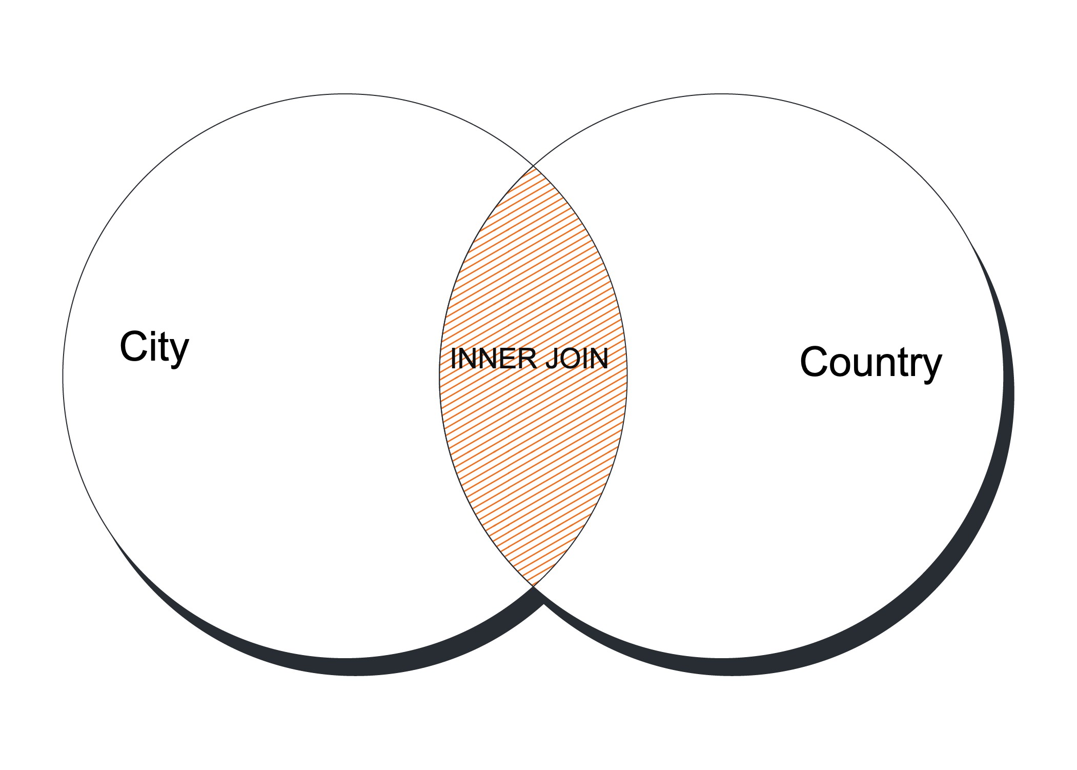
Figure 3-2. The Venn diagram representation of the INNER JOIN
As we saw in the previous example, all operators are supported when using INNER JOIN. For example, we used the WHERE condition and the LIMIT clause.
Before we leave SELECT, we’ll give you a taste of one of the functions you can use to aggregate values. Suppose you want to count how many cities Italy has in our database. You can do this by counting the number of rows using the COUNT() function. Here’s how it works:
mysql (sakila) > select count(1) FROM city INNER JOIN country ON city.country_id = country.country_id WHERE country.country_id = 49 ORDER BY country, city;----------| count(1) |----------| 7 |----------1 row in set (0.00 sec)
We explain more features of SELECT and aggregate functions in [Link to Come].
The INSERT Statement
The INSERT statement is used to add new data to tables. In this section, we explain its basic syntax and show you simple examples that add new rows to the music database. In Chapter 4, we’ll discuss how to load data from existing tables or from external data sources.
INSERT Basics
Inserting data typically occurs in two situations: when you bulk-load in a large batch as you create your database, and when you add data on an ad hoc basis as you use the database. In MySQL, there are different optimizations built into the server for each situation and, importantly, different SQL syntaxes available to make it easy for you to work with the server in both cases. We explain a basic INSERT syntax in this section, and show you examples of how to use it for bulk and single record insertion.
Let’s start with the basic task of inserting one new row into the artist table. To do this, you need to understand the table’s structure. As we explained in Chapter 2 in “The Music Database”, you can discover this with the SHOW COLUMNS statement:
mysql> SHOW COLUMNS FROM artist;-----------------------------------------------------+ | Field | Type | Null | Key | Default | Extra |-----------------------------------------------------+ | artist_id | smallint(5) | NO | PRI | 0 | | | artist_name | char(128) | NO | | | |-----------------------------------------------------+ 2 rows in set (0.00 sec)
This tells you that the two columns occur in the order artist_id and then artist_name, and you need to know this for the basic syntax we’re about to use.
Our new row is for a new artist, “Barry Adamson.” But what artist_id value do we give him? You might recall that we already have six artists, so we should probably use 7. You can check this with:
mysql> SELECT MAX(artist_id) FROM artist;----------------| MAX(artist_id) |----------------| 6 |----------------1 row in set (0.04 sec)
The MAX( ) function is an aggregate function, and it tells you the maximum value for the column supplied as a parameter. This is a little cleaner than SELECT artist_id FROM artist, which prints out all rows and requires you to inspect the rows to find the maximum value; adding an ORDER BY makes it easier. Using MAX( ) is also much simpler than SELECT artist_id FROM artist ORDER BY artist_id DESC LIMIT 1, which also returns the correct answer. You’ll learn more about the AUTO_INCREMENT shortcut to automatically assign the next available identifier in Chapter 4, and about aggregate functions in [Link to Come].
We’re now ready to insert the row. Here’s what you type:
mysql> INSERT INTO artist VALUES (7, "Barry Adamson");
Query OK, 1 row affected (0.00 sec)
A new row is created — MySQL reports that one row has been affected — and the value 7 is inserted as the artist_id and Barry Adamson as the artist_name. You can check with a query:
mysql> SELECT * FROM artist WHERE artist_id = 7;--------------------------+ | artist_id | artist_name |--------------------------+ | 7 | Barry Adamson |--------------------------+ 1 row in set (0.01 sec)
You might be tempted to try out something like this:
mysql> INSERT INTO artist

      VALUES((SELECT 1+MAX(artist_id) FROM artist), "Barry Adamson");
However, this won’t work because you can’t modify a table while you’re reading from it. The query would work if you wanted to INSERT INTO a different table (here, a table other than artist).
To continue our example, and illustrate the bulk-loading approach, let’s now insert Barry Adamson’s album The Taming of the Shrewd and its tracks. First, check the structure of the album table:
mysql> SHOW COLUMNS FROM album;--------------------------------------------------+ | Field | Type | Null | Key | Default | Extra |--------------------------------------------------+ | artist_id | int(5) | | PRI | 0 | | | album_id | int(4) | | PRI | 0 | | | album_name | char(128) | YES | | NULL | |--------------------------------------------------+ 3 rows in set (0.00 sec)
Second, insert the album using the approach we used previously:
mysql> INSERT INTO album VALUES (7, 1, "The Taming of the Shrewd");
Query OK, 1 row affected (0.00 sec)
The first value is the artist_id, the value of which we know from creating the artist, and the second value is the album_id, which must be 1 because this is the first album we’ve added for Barry Adamson.
Third, check the track table structure:
mysql> SHOW COLUMNS FROM track;-----------------------------------------------------+ | Field | Type | Null | Key | Default | Extra |-----------------------------------------------------+ | track_id | int(3) | | PRI | 0 | | | track_name | char(128) | YES | | NULL | | | artist_id | int(5) | | PRI | 0 | | | album_id | int(4) | | PRI | 0 | | | time | decimal(5,2) | YES | | NULL | |-----------------------------------------------------+ 5 rows in set (0.01 sec)
Finally, insert the tracks:
mysql> INSERT INTO track VALUES (1, "Diamonds", 7, 1, 4.10),
   -> (2, "Boppin Out / Eternal Morning", 7, 1, 3.22),
   -> (3, "Splat Goes the Cat", 7, 1, 1.39),
   -> (4, "From Rusholme With Love", 7, 1, 3.59);
Query OK, 4 rows affected (0.00 sec)
Records: 4  Duplicates: 0  Warnings: 0
Here, we’ve used a different INSERT style to add all four tracks in a single SQL query. This style is recommended when you want to load more than one row. It has a similar format to the single-insertion style, except that the values for several rows are collected together in a comma-separated list. Giving MySQL all the data you want to insert in one statement helps it optimize the insertion process, allowing queries that use this syntax to be typically many times faster than repeated insertions of single rows. There are other ways to speed up insertion, and we discuss several in Chapter 4.
The single-row INSERT style is unforgiving: if it finds a duplicate, it’ll stop as soon as it finds a duplicate key. For example, suppose we try to insert the same tracks again:
mysql> INSERT INTO track VALUES (1, "Diamonds", 7, 1, 4.10),
   -> (2, "Boppin Out / Eternal Morning", 7, 1, 3.22),
   -> (3, "Splat Goes the Cat", 7, 1, 1.39),
   -> (4, "From Rusholme With Love", 7, 1, 3.59);
ERROR 1062 (23000): Duplicate entry 7-1-1 for key 1
The INSERT operation stops on the first duplicate key. You can add an IGNORE clause to prevent the error if you want:
mysql> INSERT IGNORE INTO track VALUES (1, "Diamonds", 7, 1, 4.10),
   -> (2, "Boppin Out / Eternal Morning", 7, 1, 3.22),
   -> (3, "Splat Goes the Cat", 7, 1, 1.39),
   -> (4, "From Rusholme With Love", 7, 1, 3.59);
Query OK, 0 rows affected (0.01 sec)
Records: 4  Duplicates: 4  Warnings: 0
However, in most cases, you want to know about possible problems (after all, primary keys are supposed to be unique), and so this IGNORE syntax is rarely used.
You’ll notice that MySQL reports the results of bulk insertion differently from single insertion. From our initial bulk insertion, it reports:
Query OK, 4 rows affected (0.00 sec)
Records: 4  Duplicates: 0  Warnings: 0
The first line tells you how many rows were inserted, while the first entry in the final line tells you how many rows (or records) were actually processed. If you use INSERT IGNORE and try to insert a duplicate record — for which the primary key matches that of an existing row — then MySQL will quietly skip inserting it and report it as a duplicate in the second entry on the final line:
Query OK, 0 rows affected (0.01 sec)
Records: 4  Duplicates: 4  Warnings: 0
We discuss causes of warnings — shown as the third entry on the final line — in Chapter 4.
Alternative Syntaxes
There are several alternatives to the VALUES syntax we’ve shown you so far. This section shows you these and explains the advantages and drawbacks of each. If you’re happy with the basic syntax we’ve described so far, and want to move on to a new topic, feel free to skip ahead to “The DELETE Statement”.
There are three disadvantages of the VALUES syntax we’ve shown you. First, you need to remember the order of the columns. Second, you need to provide a value for each column. Last, it’s closely tied to the underlying table structure: if you change the table’s structure, you need to change the INSERT statements, and the function of the INSERT statement isn’t obvious unless you have the table structure at hand. However, the three advantages of the approach are that it works for both single and bulk inserts, you get an error message if you forget to supply values for all columns, and you don’t have to type in column names. Fortunately, the disadvantages are easily avoided by varying the syntax.
Suppose you know that the album table has three columns and you recall their names, but you forget their order. You can insert using the following approach:
mysql> INSERT INTO album (artist_id, album_id, album_name)
*    -> VALUES (7, 2, "Oedipus Schmoedipus");*
Query OK, 1 row affected (0.00 sec)
The column names are included in parentheses after the table name, and the values stored in those columns are listed in parentheses after the VALUES keyword. So, in this example, a new row is created and the value 7 is stored as the artist_id, 2 is stored as the album_id, and Oedipus Schmoedipus is stored as the album_name. The advantages of this syntax are that it’s readable and flexible (addressing the third disadvantage we described) and order-independent (addressing the first disadvantage). The disadvantage is that you need to know the column names and type them in.
This new syntax can also address the second disadvantage of the simpler approach — that is, it can allow you to insert values for only some columns. To understand how this might be useful, let’s explore the played table:
mysql> SHOW COLUMNS FROM played;-----------------------------------------------------------+ | Field | Type | Null | Key | Default | Extra |-----------------------------------------------------------+ | artist_id | int(5) | | PRI | 0 | | | album_id | int(4) | | PRI | 0 | | | track_id | int(3) | | PRI | 0 | | | played | timestamp | YES | PRI | CURRENT_TIMESTAMP | |-----------------------------------------------------------+ 4 rows in set (0.00 sec)
Notice that the played column has a default value of CURRENT_TIMESTAMP. This means that if you don’t insert a value for the played column, it’ll insert the current date and time by default. This is just what we want: when we play a track, we don’t want to bother checking the date and time and typing it in. Here’s how you insert an incomplete played entry:
mysql> INSERT INTO played (artist_id, album_id, track_id)
   -> VALUES (7, 1, 1);
Query OK, 1 row affected (0.00 sec)
We didn’t set the played column, so MySQL defaults it to the current date and time. You can check this with a query:
mysql> SELECT * FROM played WHERE artist_id = 7 -> AND album_id = 1;----------------------------------------------------+ | artist_id | album_id | track_id | played |----------------------------------------------------+ | 7 | 1 | 1 | 2006-08-09 12:03:00 |----------------------------------------------------+ 1 row in set (0.00 sec)
You can also use this approach for bulk insertion as follows:
mysql> INSERT INTO played (artist_id, album_id, track_id)
   -> VALUES (7,1,2),(7,1,3),(7,1,4);
Query OK, 3 rows affected (0.00 sec)
Records: 3  Duplicates: 0  Warnings: 0
The disadvantages of this approach are that you can accidentally omit values for columns, and you need to remember and type column names. The omitted columns will be set to the default values.
All columns in a MySQL table have a default value of NULL unless another default value is explicitly assigned when the table is created or modified. Because of this, defaults can often cause duplicate rows: if you add a row with the default primary key values and repeat the process, you’ll get a duplicate error. However, the default isn’t always sensible; for example, in the played table, the artist_id, album_id, and track_id columns all default to 0, which doesn’t make sense in the context of our music collection. Let’s try adding a row to played with only default values:
mysql> INSERT INTO played () VALUES ();
Query OK, 1 row affected (0.00 sec)
The ( ) syntax is used to represent that all columns and values are to be set to their defaults. Let’s find our new row by asking for the most recent played time:
mysql> SELECT * FROM played ORDER BY played DESC LIMIT 1;----------------------------------------------------+ | artist_id | album_id | track_id | played |----------------------------------------------------+ | 0 | 0 | 0 | 2006-08-09 12:20:40 |----------------------------------------------------+ 1 row in set (0.00 sec)
The process worked, but the row doesn’t make any sense. We’ll discuss default values further in Chapter 4.
You can set defaults and still use the original INSERT syntax with MySQL 4.0.3 or later by using the DEFAULT keyword. Here’s an example that adds a played row:
mysql> INSERT INTO played VALUES (7, 1, 2, DEFAULT);
Query OK, 1 row affected (0.00 sec)
The keyword DEFAULT tells MySQL to use the default value for that column, and so the current date and time are inserted in our example. The advantages of this approach are that you can use the bulk-insert feature with default values, and you can never accidentally omit a column.
There’s another alternative INSERT syntax. In this approach, you list the column name and value together, giving the advantage that you don’t have to mentally map the list of values to the earlier list of columns. Here’s an example that adds a new row to the played table:
mysql> INSERT INTO played
   -> SET artist_id = 7, album_id = 1, track_id = 1;
Query OK, 1 row affected (0.00 sec)
The syntax requires you list a table name, the keyword SET, and then column-equals-value pairs, separated by commas. Columns that aren’t supplied are set to their default values. The disadvantages are again that you can accidentally omit values for columns, and that you need to remember and type in column names. A significant additional disadvantage is that you can’t use this method for bulk insertion.
You can also insert using values returned from a query. We discuss this in [Link to Come].
The DELETE Statement
The DELETE statement is used to remove one or more rows from a database. We explain single-table deletes here, and discuss multi-table deletes — which remove data from two or more tables through one statement — in [Link to Come].
If you want to try out the steps in this section on your MySQL server, you’ll need to reload your music database afterwards so that you can follow the examples in later sections. To do this, follow the steps you used in [Link to Come] in [Link to Come] to load it in the first place.
DELETE Basics
The simplest use of DELETE is to remove all rows in a table. Suppose you want to empty your played table, perhaps because it’s taking too much space or because you want to share your music database with someone else and they don’t want your played data. You do this with:
mysql> DELETE FROM played;
Query OK, 19 rows affected (0.07 sec)
This removes all rows, including those we just added in “The INSERT Statement”; you can see that 19 rows have been affected.
The DELETE syntax doesn’t include column names, since it’s used to remove whole rows and not just values from a row. To reset or modify a value in a row, you use the UPDATE statement, described later in this chapter in “The UPDATE Statement”. The DELETE statement doesn’t remove the table itself. For example, having deleted all rows in the played table, you can still query the table:
mysql> SELECT * FROM played;
Empty set (0.00 sec)
Of course, you can also continue to explore its structure using DESCRIBE or SHOW CREATE TABLE, and insert new rows using INSERT. To remove a table, you use the DROP statement described in Chapter 4.
Using WHERE, ORDER BY, and LIMIT
If you’ve deleted rows in the previous section, reload your music database now. You need the rows in the played table restored for the examples in this section.
To remove one or more rows, but not all rows in a table, you use a WHERE clause. This works in the same way as it does for SELECT. For example, suppose you want to remove all rows from the played table with played dates and times earlier than August 15, 2006. You do this with:
mysql> DELETE FROM played WHERE played < "2006-08-15";
Query OK, 8 rows affected (0.00 sec)
The result is that the eight played rows that match the criteria are removed. Note that the date is enclosed in quotes and that the date format is year, month, day, separated by hyphens. MySQL supports several different ways of specifying times and dates but saves dates in this internationally friendly, easy-to-sort format (it’s actually an ISO standard). MySQL can also reasonably interpret two-digit years, but we recommend against using them; remember all the work required to avoid the Y2K problem?
Suppose you want to remove an artist, his albums, and his album tracks. For example, let’s remove everything by Miles Davis. Begin by finding out the artist_id from the artist table, which we’ll use to remove data from all four tables:
mysql> SELECT artist_id FROM artist WHERE artist_name = "Miles Davis";-----------| artist_id |-----------| 3 |-----------1 row in set (0.00 sec)
Next, remove the row from the artist table:
mysql> DELETE FROM artist WHERE artist_id = 3;
Query OK, 1 row affected (0.00 sec)
Then, do the same thing for the album, track, and played tables:
mysql> DELETE FROM album WHERE artist_id = 3;
Query OK, 2 rows affected (0.01 sec)

mysql> DELETE FROM track WHERE artist_id = 3;
Query OK, 13 rows affected (0.01 sec)

mysql> DELETE FROM played WHERE artist_id = 3;
Query OK, 3 rows affected (0.00 sec)
Since all four tables can be joined using the artist_id column, you can accomplish this whole deletion process in a single DELETE statement; we show you how in [Link to Come].
You can use the ORDER BY and LIMIT clauses with DELETE. You usually do this when you want to limit the number of rows deleted, either so that the statement doesn’t run for too long or because you want to keep a table to a specific size. Suppose your played table contains 10,528 rows, but you want to have at most 10,000 rows. In this situation, it may make sense to remove the 528 oldest rows, and you can do this with the following statement:
mysql> DELETE FROM played ORDER BY played LIMIT 528;
Query OK, 528 rows affected (0.23 sec)
The query sorts the rows by ascending play date and then deletes at most 528 rows, starting with the oldest. Typically, when you’re deleting, you use LIMIT and ORDER BY together; it usually doesn’t make sense to use them separately. Note that sorting large numbers of entries on a field that doesn’t have an index can be quite slow. We discuss indexes in detail in “Keys and Indexes” in Chapter 4.
Removing All Rows with TRUNCATE
If you want to remove all rows in a table, there’s a faster method than removing them with DELETE. By using the TRUNCATE TABLE statement, MySQL takes the shortcut of dropping the table — that is, removing the table structures and then re-creating them. When there are many rows in a table, this is much faster.
If you want to remove the data in the played table, you can write this:
mysql> TRUNCATE TABLE played;
Query OK, 0 rows affected (0.00 sec)
Notice that the number of rows affected is shown as zero: to quickly delete all the data in the table, MySQL doesn’t count the number of rows that are deleted, so the number shown (normally zero, but sometimes nonzero) does not reflect the actual number of rows deleted.
The TRUNCATE TABLE statement has two other limitations:
-
It’s actually identical to
DELETEif you use InnoDB tables. -
It does not work with locking or transactions.
Table types, transactions, and locking are discussed in [Link to Come]. In practice, none of these limitations affect most applications, and you can use TRUNCATE TABLE to speed up your processing. Of course, it’s not common to delete whole tables during normal operation. An exception is temporary tables, which are used to temporarily store query results for a particular user session and can be deleted without losing the original data.
The UPDATE Statement
The UPDATE statement is used to change data. In this section, we show you how to update one or more rows in a single table. Multitable updates are discussed in [Link to Come].
If you’ve deleted rows from your music database, reload it by following the instructions in [Link to Come] in [Link to Come]. You need a copy of the unmodified music database to follow the examples in this section.
Examples
The simplest use of the UPDATE statement is to change all rows in a table. There isn’t much need to change all rows from a table in the music database — any example is a little contrived — but let’s do it anyway. To change the artist names to uppercase, you can use:
mysql> UPDATE artist SET artist_name = UPPER(artist_name);
Query OK, 6 rows affected (0.04 sec)
Rows matched: 6  Changed: 6  Warnings: 0
The function UPPER( ) is a MySQL function that returns the uppercase version of the text passed as the parameter; for example, New Order is returned as NEW ORDER. You can see that all six artists are modified, since six rows are reported as affected. The function LOWER( ) performs the reverse, converting all the text to lowercase.
The second row reported by an UPDATE statement shows the overall effect of the statement. In our example, you see:
Rows matched: 6 Changed: 6 Warnings: 0
The first column reports the number of rows that were retrieved as answers by the statement; in this case, since there’s no WHERE or LIMIT clause, all six rows in the table match the query. The second column reports how many rows needed to be changed, and this is always equal to or less than the number of rows that match; in this example, since none of the strings are entirely in uppercase, all six rows are changed. If you repeat the statement, you’ll see a different result:
mysql> UPDATE artist SET artist_name = UPPER(artist_name);
Query OK, 0 rows affected (0.00 sec)
Rows matched: 6  Changed: 0  Warnings: 0
This time, since all of the artists are already in uppercase, six rows still match the statement but none are changed. Note also the number of rows changed is always equal to the number of rows affected, as reported on the first line of the output.
Our previous example updates each value relative to its current value. You can also set columns to a single value. For example, if you want to set all played dates and times to the current date and time, you can use:
mysql> UPDATE played SET played = NULL;
Query OK, 11 rows affected (0.00 sec)
Rows matched: 11  Changed: 11  Warnings: 0
You’ll recall from “Alternative Syntaxes” that since the default value of the played column is CURRENT_TIMESTAMP, passing a NULL value causes the current date and time to be stored instead. Since all rows match and all rows are changed (affected), you can see three 11s in the output.
Using WHERE, ORDER BY, and LIMIT
Often, you don’t want to change all rows in a table. Instead, you want to update one or more rows that match a condition. As with SELECT and DELETE, the WHERE clause is used for the task. In addition, in the same way as with DELETE, you can use ORDER BY and LIMIT together to control how many rows are updated from an ordered list.
Let’s try an example that modifies one row in a table. If you browse the album database, you’ll notice an inconsistency for the two albums beginning with “Substance”:
mysql> SELECT * FROM album WHERE album_name LIKE -> "Substance%";----------------------------------------------| artist_id | album_id | album_name |----------------------------------------------| 1 | 2 | Substance (Disc 2) | | 1 | 6 | Substance 1987 (Disc 1) |----------------------------------------------2 rows in set (0.00 sec)
They’re actually part of the same two CD set, and the first-listed album is missing the year 1987, which is part of the title. To change it, you use an UPDATE command with a WHERE clause:
mysql> UPDATE album SET album_name = "Substance 1987 (Disc 2)"
   -> WHERE artist_id = 1 AND album_id = 2;
Query OK, 1 row affected (0.01 sec)
Rows matched: 1  Changed: 1  Warnings: 0
As expected, one row was matched, and one row was changed.
To control how many updates occur, you can use the combination of ORDER BY and LIMIT. As with DELETE, you would do this because you either want the statement to run for a controlled amount of time, or you want to modify only some rows. Suppose you want to set the 10 most recent played dates and times to the current date and time (the default). You do this with:
mysql> UPDATE played SET played = NULL ORDER BY played DESC LIMIT 10;
Query OK, 10 rows affected (0.00 sec)
Rows matched: 10  Changed: 10  Warnings: 0
You can see that 10 rows were matched and were changed.
The previous query also illustrates an important aspect of updates. As you’ve seen, updates have two phases: a matching phase — where rows are found that match the WHERE clause — and a modification phase, where the rows that need changing are updated. In our previous example, the ORDER BY played is used in the matching phase, to sort the data after it’s read from the table. After that, the modification phase processes the first 10 rows, updating those that need to be changed. Since MySQL 4.0.13, the LIMIT clause controls the maximum number of rows that are matched. Prior to this, it controlled the maximum number of rows that were changed. The new implementation is better; under the old scheme, you had little control over the update processing time when many rows matched but few required changes.
Exploring Databases and Tables with SHOW and mysqlshow
We’ve already explained how you can use the SHOW command to obtain information on the structure of a database, its tables, and the table columns. In this section, we’ll review the most common types of SHOW statement with brief examples using the music database. The mysqlshow command-line program performs the same function as several SHOW command variants, but without needing to start the monitor.
The SHOW DATABASES statement lists the databases you can access. If you’ve followed our sample database installation steps in [Link to Come] in [Link to Come], your output should be as follows:
mysql> show databases;--------------------| Database |--------------------| information_schema | | mysql | | performance_schema | | sakila | | sys | | test |--------------------6 rows in set (0.01 sec)
These are the databases that you can access with the USE command; as we explain in [Link to Come], you can’t see databases for which you have no access privileges unless you have the global SHOW DATABASES privilege. You can get the same effect from the command line using the mysqlshow program:
bash> mysqlshow -uroot -pmsandbox -h 127.0.0.1 -P 3306
You can add a LIKE clause to SHOW DATABASES. This is useful only if you have many databases and want a short list as output. For example, to see databases beginning with m, type:
mysql> show databases like s%;---------------| Database (s%) |---------------| sakila | | sys |---------------2 rows in set (0.00 sec)
The syntax of the LIKE statement is identical to that in its use in SELECT.
To see the statement used to create a database, you can use the SHOW CREATE DATABASE statement. For example, to see how sakila was created, type:
mysql > show create database sakila;--------------------------------------------------------------------------------------------------------------------------------------------+ | Database | Create Database |--------------------------------------------------------------------------------------------------------------------------------------------+ | sakila | CREATE DATABASE `sakila` /!40100 DEFAULT CHARACTER SET utf8mb4 COLLATE utf8mb4_0900_ai_ci */ /!80016 DEFAULT ENCRYPTION=N */ |--------------------------------------------------------------------------------------------------------------------------------------------+ 1 row in set (0.00 sec)
This is perhaps the least exciting SHOW statement; it only displays the statement:
CREATE DATABASE `sakila` /*!40100 DEFAULT CHARACTER SET utf8mb4 COLLATE utf8mb4_0900_ai_ci */ /*!80016 DEFAULT ENCRYPTION='N' */
There are some additional keywords that are enclosed between the comment symbols 0! and 1:
40100 DEFAULT CHARACTER SET utf8mb4 COLLATE utf8mb4_0900_ai_ci
80016 DEFAULT ENCRYPTION='N'
These instructions contain MySQL-specific extensions to standard SQL that are unlikely to be understood by other database programs. A database server other than MySQL would ignore this comment text, and so the syntax is usable by both MySQL and other database server software. The optional number 40100 indicates the minimum version of MySQL that can process this particular instruction — in this case, version 4.01.00; older versions of MySQL ignore such instructions. You’ll learn about creating databases in Chapter 4.
The SHOW TABLES statement lists the tables in a database. To check the tables in sakila, type:
mysql> show tables from sakila;----------------------------| Tables_in_sakila |----------------------------| actor | | actor_info | | address | | category | | city | | country | | customer | | customer_list | | film | | film_actor | | film_category | | film_list | | film_text | | inventory | | language | | nicer_but_slower_film_list | | payment | | rental | | sales_by_film_category | | sales_by_store | | staff | | staff_list | | store |----------------------------23 rows in set (0.01 sec)
If you’ve already selected the sakila database with the USE sakila command, you can use the shortcut:
mysql> SHOW TABLES;
You can get a similar result by specifying the database name to the mysqlshow program:
$ mysqlshow -uroot -pmsandbox -h 127.0.0.1 -P 3306 sakila
As with SHOW DATABASES, you can’t see tables that you don’t have privileges for. This means you can’t see tables in a database you can’t access, even if you have the SHOW DATABASES global privilege.
The SHOW COLUMNS statement lists the columns in a table. For example, to check the columns of country, type:
mysql (sakila) > show columns from country;-------------------------------------------------------------------------------------------------------------+ | Field | Type | Null | Key | Default | Extra |-------------------------------------------------------------------------------------------------------------+ | country_id | smallint unsigned | NO | PRI | NULL | auto_increment | | country | varchar(50) | NO | | NULL | | | last_update | timestamp | NO | | CURRENT_TIMESTAMP | DEFAULT_GENERATED on update CURRENT_TIMESTAMP |-------------------------------------------------------------------------------------------------------------+ 3 rows in set (0.00 sec)
The output reports all column names, their types and sizes, whether they can be NULL, whether they are part of a key, their default value, and any extra information. Types, keys, NULL values, and defaults are discussed further in Chapter 4. If you haven’t already chosen the sakila database with the USE command, then you can add the database name before the table name, as in sakila.country. Unlike the previous SHOW statements, you can always see all column names if you have access to a table; it doesn’t matter that you don’t have certain privileges for all columns. You can get a similar result by using mysqlshow with the database and table name:
$ mysqlshow -uroot -pmsandbox -h 127.0.0.1 -P 3306 sakila country
And you will receive:
Database: sakila Table: country---------------------------------------------------------------------------------------------------------------------------------------------------------------------------| Field | Type | Collation | Null | Key | Default | Extra | Privileges | Comment |---------------------------------------------------------------------------------------------------------------------------------------------------------------------------| country_id | smallint unsigned | | NO | PRI | | auto_increment | select,insert,update,references | | | country | varchar(50) | utf8mb4_0900_ai_ci | NO | | | | select,insert,update,references | | | last_update | timestamp | | NO | | CURRENT_TIMESTAMP | DEFAULT_GENERATED on update CURRENT_TIMESTAMP | select,insert,update,references | |---------------------------------------------------------------------------------------------------------------------------------------------------------------------------
You can see the statement used to create a particular table using the SHOW CREATE TABLE statement; creating tables is a subject of Chapter 4. Some users prefer this output to that of SHOW COLUMNS, since it has the familiar format of a CREATE TABLE statement. Here’s an example for the country table:
mysql (sakila) > SHOW CREATE TABLE countryG
 1. row
       Table: country
Create Table: CREATE TABLE `country` (
  `country_id` smallint unsigned NOT NULL AUTO_INCREMENT,
  `country` varchar(50) NOT NULL,
  `last_update` timestamp NOT NULL DEFAULT CURRENT_TIMESTAMP ON UPDATE CURRENT_TIMESTAMP,
  PRIMARY KEY (`country_id`)
) ENGINE=InnoDB AUTO_INCREMENT=110 DEFAULT CHARSET=utf8mb4 COLLATE=utf8mb4_0900_ai_ci
1 row in set (0.00 sec)