
CHAPTER 9
Some Powerful Methods Based on Bayes
If one fails to specify the prior information, a problem of inference is just as ill‐posed as if one had failed to specify the data … In realistic problems of inference, it is typical that we have cogent prior information, highly relevant to the question being asked; to fail to take it into account is to commit the most obvious inconsistency of reasoning, and it may lead to absurd or dangerously misleading results.
—Edwin T. Jaynes
Recall that in our survey, 23% of respondents agreed with the statement “Probabilistic methods are impractical because probabilities need exact data to be computed and we don't have exact data.” This is just a minority, but even those who rejected that claim probably have found themselves in situations where data seemed too sparse to make a useful inference. In fact, that may be why the majority of the survey takers also responded that ordinal scales have a place in measuring uncertainty. Perhaps they feel comfortable using wildly inexact and arbitrary values such as “high, medium, and low” to communicate risk while, ironically, still believing in quantitative approaches. Yet someone who thoroughly believed in using quantitative methods would have roundly rejected ordinal scales when measuring highly uncertain events. When you are highly uncertain you use probabilities and ranges to actively communicate your uncertainty—particularly when you are relying on subject matter expertise. Having read the earlier research in this book, you know how even subjective estimates can be decomposed and made more consistent before any new “objective” data is applied and how even a single data point (such as the outcome of one penetration test) can be used to update that belief.
Now that we've laid some groundwork of Bayesian empirical methods with an (admittedly) oversimplified example, we can show solutions to slightly more advanced—and more realistic—problems.
Computing Frequencies with (Very) Few Data Points: The Beta Distribution
There are some slightly more elaborate derivatives of Bayes's rule that should come up frequently in cybersecurity. Let's say you are one of the big retailers we discussed in Chapter 6, and again we would like to assess the probability of a major data breach. Our new empirical data is widely publicized, major data breaches. Of course, you would like to leverage these news reports to estimate the chance that your firm would have such a breach.
In a perfect world, you would have the equivalent cybersecurity version of an actuarial table as used in insurance products such as life, health, and property. You would have thousands of firms in your own industry diligently reporting data points over many decades. You would use this to compute a data breach “rate” or “frequency.” This is expressed as the percentage of firms that will have a data breach in a given year. As in insurance, we would use that as a baseline for the chance of your firm having such an event.
If you only have publicized examples from your own industry, you may not have that many data points. Fortunately, we may need less data than we think if we use a particular statistical tool known as the “beta” distribution. With the beta distribution, we can make an inference about this annualized rate of a breach even with what seems like very little data.
So you need less data than you think and, as we first said in Chapter 2, you also have more data than you think. In the case of reputation loss, for example, saying that we lack data about major data breaches is curious since we actually have all the data. That is, every major, large‐retail data breach with massive costs that has occurred was public. Many of the costs are, in fact, because it was widely publicized. If there was a major data breach that was somehow not public, then that retailer has, so far, avoided some or most of the main costs of a breach.
If we look at the Verizon Data Breach Investigations Report (DBIR) and other sources of data on breaches, we can see a number of breaches in each industry. But that information alone doesn't tell us what the probability of a breach is for a single firm in a given industry. If there were five breaches in a given industry in a given year, is that five out of 20 (25%) of the industry or five out of 100 (5%)? If we want to estimate the chance that a given firm (yours) will have a publicized data breach in the next year, we need to know the size of the population those firms were drawn from, including those that didn't have breaches.
Now, this is where some cybersecurity experts, who recall just enough stats to get it all wrong, will give up on this by saying that the few breaches are not “statistically significant” and that no inferences could be made. Others—especially those, we hope, who have read this book—will not give up so easily on such an important question for their organization.
Calculations with the Beta Distribution
The beta distribution is useful when you are trying to estimate a population proportion. A population proportion is just the share of a population that falls in some subset. If only 25% of employees are following a procedure correctly, then the “25%” refers to a population proportion. If we could conduct a complete census of the population, we would know the proportion exactly. But you may only have access to a small sample. If we were only able to randomly sample, say, 10 people of a population of thousands of employees, would that tell us anything? This is where the beta distribution comes in. And you may be surprised to find that, according to the beta distribution, we may not need very many samples to tell us something we didn't know already.
This would apply to many situations in cybersecurity, including the likelihood of a risk that relatively few organizations have experienced. A beta distribution has just two parameters that seem at first to be a little abstract: alpha and beta (we will explain them shortly). In Excel we write this as =betadist(x,alpha,beta), where x is the population proportion you want to test. The formula produces the probability that the population proportion is less than x—we call this the “cumulative probability function” (cpf) since for each x it gives the cumulative probability up to that point.
There is also an “inverse probability function” in Excel for the beta distribution, written as =beta.inv(p,alpha,beta), where p is a probability, and the formula returns the population proportion just high enough such that there is a p probability that the true population proportion is lower.
Many stats texts don't offer a concrete way to think about what alpha and beta represent, yet there is an intuitive way to think about it. Just think of alpha and beta as “hits” and “misses” in a sample. A “hit” in a sample is, say, an employee following a procedure correctly and a “miss” is one who is not.
To compute alpha and beta from hits and misses we need to establish our prior probability. Again, an informative prior probability could simply be a calibrated subject‐matter expert (SME) estimate. They might estimate a 90% CI that between 10% and 40% of all staff follow this procedure correctly. But if we want to be extremely conservative, we can use what is called an “uninformative prior” by simply using a uniform distribution of 0% to 100%.
In a beta distribution, we represent an uninformative uniform prior by setting both alpha and beta to a value of 1. Think of it as a “free hit” and a “free miss” you get with each beta distribution. This approach indicates we have almost no information about what a true population proportion could be. All we know is the mathematical constraint that a proportion of a population can't be less than 0% and can't exceed 100%. Note that this can't be a 90% CI as the calibrated SME provided since there is no chance of being outside that range. It represents the minimum and maximum possible values. Other than that, we're simply saying everything in between is equally likely, as shown in Figure 9.1.
Note that this figure shows the uniform distribution in the more familiar “probability density function” (pdf) where the area under the curve adds up to 1. Since the betadist() function is a cumulative probability, we have to slice up a bunch of increments by computing the difference between two cumulative probability functions close to each other. Just think of the height of a point on a pdf to represent the relative likelihood compared to other points. Recall that a normal distribution is highest in the middle. This just means that values near the middle of a normal distribution are more likely. In the case of this uniform distribution, we show that all values between the min and max are equally likely (i.e., it is flat).

FIGURE 9.1 A Uniform Distribution (a Beta Distribution with alpha=beta=1)
Now, if we have a sample of some population, even a very small sample, we can update the alpha and beta with a count of hits and misses. Again, consider the case where we want to estimate the share of users following certain security procedures. We randomly sample six and find that only one is doing it correctly. Let's call the one a “hit” and the remaining five “misses.” We simply add hits to our prior alpha and misses to our prior beta to get:

FIGURE 9.2 A Distribution Starting with a Uniform Prior and Updated with a Sample of 1 Hit and 5 Misses
Figure 9.2 shows what a pdf would look like if we added a sample of six with one “hit” to our prior uniform distribution. To create this picture you can use the calculation below:

where “i” is the size of an increment we are using (the increment size is arbitrary, but the smaller you make it the finer detail you get in your pictures of distributions). One hit out of a sample of six gives us a 90% CI of 5.3% to 52%. Again, you have an example in the spreadsheet in www.howtomeasureanything.com/cybersecurity to do this calculation.
How does the beta distribution do this? Doesn't this contradict what we learned in first semester statistics about sample sizes? No. The math is sound. In effect, the beta distribution applies Bayes's rule over a range of possible values. To see how this works, consider a trivial question such as “What is the probability of getting 1 hit out of 6 samples if only 1% of the population were following the procedure correctly?” If we assume we know a population proportion and we want to work out the chance of getting so many “hits” in a sample, we apply something called a binomial distribution.
The binomial distribution is a kind of complement to the beta distribution. In the former, you estimate the probabilities of different sample results given the population proportion. In the latter, you estimate the population proportion given a number of sample results. In Excel, we write the binomial distribution as =binomdist(hits,samplesize,probability,0). (The “0” means it will produce the probability of that exact outcome, not the cumulative probability up to that point.)
This would give us the chance of getting the observed result (e.g., 1 out of 6) for one possible population proportion (in this case 1%). We repeat this for a hypothetical population proportion of 2%, 3%, and so on up to 100%. Now Bayes lets us flip this into what we really want to know: “What is the probability of X being the population proportion given that we had 1 hit out of 6?” In other words, the binomial distribution gave us P(observed data|proportion) and we flip it to P(proportion|observed data). This is a neat trick that will be very useful, and it is already done for us in the beta distribution.
One more thing before we move on: Does 5.3% to 52% seem like a wide range? Well, remember you only sampled six people. And your previous range was even wider (on a uniform distribution of 0% to 100%, a 90% CI is 5% to 95%). All you need to do to keep reducing the width of this range is to keep sampling and each sample will slightly modify your range. You could have gotten a distribution even if you had zero hits out of three samples as long as you started with a prior.
If you need another example to make this concrete, let's consider one Hubbard uses in How to Measure Anything. Imagine you have an urn filled with red and green marbles. Let's say you think the proportion of red marbles could be anywhere between 0% and 100% (this is your prior). To estimate the population proportion, you sample 6 marbles, one of which was red. We would estimate the result as we did in the security procedure example above—the range would be 5.3% to 52%. The reason this range is wide is because we know we could have gotten 1 red out of 6 marbles from many possible population proportions. We could have gotten that result if just, say, 7% were red and we could have gotten that result if half were red.
Applying the Beta to Breaches
Imagine that every firm in your industry is randomly drawing from the “breach urn” every year. Some firms draw a red marble, indicating they were breached. But there could have been more, and there could have been less. You don't really know breach frequency (i.e., the portion of marbles that are red). But you can use the observed breaches to estimate the proportion of red marbles. Note that we are making a simplifying assumption that an event either occurs in a given year or not. We will ignore, for now, the possibility that it could happen multiple times per year. (When the probability per year is less than about 10%, this assumption is not far off the mark.)
For a source of data, we could start with a list of reported breaches from the DBIR. However, the DBIR itself doesn't usually tell us the size of the population. This is sort of like knowing there are 100 red marbles in the urn but without knowing the total number of marbles we can't know the population proportion of red marbles. However, we could still randomly sample a set of marbles and just use the number of red marbles in that sample compared to the size of the sample instead of the unknown total population size. Likewise, knowing that there were X breaches in our industry only helps if we know the size of the industry. So we find another source—not the DBIR—for a list of retailers. It could be the retailers in the Fortune 500 or perhaps a list from a retailers association. That list should have nothing to do with whether an organization had a breach reported in the DBIR, so many of those in that list will not have been mentioned in the DBIR. That list is our sample (how many marbles we draw from the urn). Some of those, however, will be mentioned in the DBIR as having experienced a breach (i.e., drawing a red marble).
Let's say we found 60 retailers in an industry list that would be relevant to you. Of that sample of 60, you find that in the time period between the start of 2021 and the end of 2022, there were two reported major data breaches. Since we are estimating a per‐year chance of a breach, we have to multiply the number of years in our data by the number of firms. To summarize:
- Sample Size: 120 company‐years of data (60 firms × 2 years);
- Hits: 2 breaches in that time period;
- Misses: 118 company‐years where there was no major breach;
- Alpha: prior + hits = 1 + 2 = 3;
- Beta: prior + misses = 1 + 118 = 119.
When we plug this into our spreadsheet we get a distribution like the one shown in Figure 9.3.

FIGURE 9.3 The Per‐Year Frequency of Data Breaches in This Industry
Think of the observed breaches as a sample of what could have happened. Just because we drew 120 marbles and two of them were red, that doesn't mean that exactly 1.67% of the marbles in the urn were red. If we drew that from the urn, we would estimate that there is a 90% chance that the true population proportion of red marbles in the urn is in the range 0.7% to 5.1%. Likewise, just because we had two breaches out of 60 firms in two years (120 company years) doesn't mean we treat the per‐year annual breach frequency as exactly 1.67%. We are only estimating the probability of different frequencies from a few observations. Next year we could be more lucky or less lucky even if the long‐term frequency is no different.
Even the mean of the beta distribution isn't exactly 1.67% since the mean of a beta distribution is alpha/(alpha + beta) or 2.46%. The reason these are different is because the beta distribution is affected by your prior. Even if there were no breaches, the beta would have an alpha of 1 and a beta of 121 (120 misses + 1 for the prior beta), giving us a mean of 0.8%.
Another handy feature of the beta distribution is how easily it is updated. Every year that goes by—in fact every day that goes by—either with or without data breaches can update the alpha and beta of a distribution of breaches in your relevant industry population. For every firm where an event occurred in that period we update the alpha, and for every firm where it didn't occur we update the beta parameter. Even if we observe no events for a whole year, we still update the beta parameters and, therefore, our assessment of the probability of the event.
Note that you don't have to use an uninformative prior such as a uniform distribution. If you have reason to believe, even before reviewing new data, that some frequencies are much less likely than others, then you can say so. You can make up a prior of any shape you like by trying different alphas and betas until you get the distribution you think fits your prior. You can start finding your prior by starting with alpha and beta equal to 1 and then, if you think the frequency is closer to zero, add to beta. Keep in mind the mean you want must be alpha/(alpha + beta). You can also add to alpha to move the frequency a little further away from zero. The larger the total alpha + beta, the narrower your range will be. Test your range by using the inverse probability function for beta in Excel: =beta.inv(.05,alpha,beta) and =beta.inv(.95,alpha,beta) will be your 90% confidence interval. After that, updating your distribution based on new information follows the same procedure—add hits to alpha and misses to beta.
The Effect of the Beta Distribution on Your Model
If we didn't use the beta distribution and instead took the observed frequency of 1.67% literally, we could be seriously underestimating risks for this industry. If we were drawing from an urn that we knew was exactly 1.67% red marbles (the rest are green), then we would still expect variation from draw to draw. If we drew 120 marbles, and assumed that the proportion of red marbles was 1.67%, we can compute that there is only a 14% chance that we would draw more than three red marbles using the formula in Excel: 1−binomdist(3,120,.0167,1). On the other hand, if we merely had a 90% CI that 0.7% to 5.1% are red, instead of the exact proportion of 1.67%, then the chance of drawing more than three red marbles increases to over 33%.
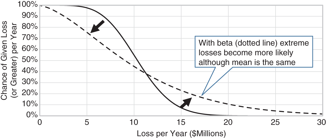
FIGURE 9.4 Example of How a Beta Distribution Changes the Chance of Extreme Losses
If we apply this thinking to security risks in an industry or a firm, the chance of multiple events increases dramatically. This could mean a higher chance in one year of multiple major breaches in the industry or, using data at the company level, multiple systems compromised out of a portfolio of many systems. In effect, this “rotates” our loss exceedance curve (LEC) counterclockwise as shown in Figure 9.4. The mean is held constant while the risk of more extreme losses increases. This may mean that your risk tolerance is now exceeded on the right end of the curve.
We believe this may be a major missing component of risk analysis in cybersecurity. We can realistically only treat past observations as a sample of possibilities and, therefore, we have to allow for the chance that we were just lucky in the past.
To see how we worked this out in detail, and to see how a beta distribution can be used in the simple one‐for‐one substitution and how it might impact the loss exceedance curve, just download the spreadsheet for this chapter on the website.
A Beta Distribution Case: AllClear ID
AllClear ID, a leading firm in customer‐facing breach response in the cybersecurity ecosystem, uses a beta distribution to estimate cybersecurity risks using industry breach data. The company offers three solutions: AllClear Reserved Response™, Customer Communication services that include customer support and notification, and Identity Protection services for consumers. They handle incidents of all sizes including some of the biggest data breaches that have happened in recent history.
The capacity to respond to incidents is guaranteed for Reserved Response clients, making risk estimation critical to ensuring adequate resources are in place to meet service requirements. In 2015, AllClear ID contacted Doug Hubbard's firm, Hubbard Decision Research, to model the data breach risks in all of the industries they support, including the chance that multiple large clients could experience breaches in overlapping periods of time. This model is one of the many tools used by AllClear ID in their risk estimation analysis.
HDR applied the beta distribution to industry breach data in the Verizon Data Breach Investigations Report (DBIR). There were 2,435 data breaches reported in the 2015 DBIR but, as we explained earlier in this chapter, this alone does not tell us the per‐year frequency of breaches for a given number of firms. Applying the same method explained earlier, we started with a known list of firms from the industries AllClear ID supports. We then cross‐referenced that with the DBIR data to determine how many of those had breaches. In the case of one industry, there were 98 firms in the Fortune 500 list. Of those, several had a breach in the two‐year period between the beginning of 2014 and the end of 2015. So 98 organizations over a two‐year period give us a total of 196 organization‐years of data where there were “hits” and “misses” (misses are firms that did not have a breach in a year). Now we can estimate the probability of a breach for the Fortune 500 firms in that industry.
In a Monte Carlo simulation, HDR used a beta distribution to produce a 90% confidence interval for the annual frequency of events per client. If the rate of breaches is at the upper bound, then the chance of multiple client breaches overlapping goes up considerably. The Monte Carlo model showed there is a chance that the peak activity period of multiple Reserved Response clients would overlap. This knowledge is one input to help AllClear ID to plan for the resources needed to meet the needs of clients even though the exact number and timing of breaches cannot be known with certainty.
Although breaches are unpredictable events, the simulation gave us invaluable insight into the risks we could potentially encounter and the intelligence to help mitigate those risks.
—Bo Holland, Founder & CEO of AllClear ID
Laplace and Beta
In the urn example, we were working out the CI for a population proportion of red marbles given a few random samples of marbles. This is analogous to estimating a proportion of staff using a procedure correctly. In some situations, we would like the answer to a different question: What is the chance that the next marble we draw will be red? Or, in the case of data breaches, what is the chance that your particular firm will experience a data breach in the next year given what we observed in many firms over multiple years?
If we knew that exactly 30% of the marbles in the urn were red, we would know that there is a 30% chance that the next marble we draw will be red. Now suppose we had two urns where one was 30% red, the other was 10% red, and we didn't know which urn we drew from. If we say that either urn is equally likely to be the one we draw from, then we compute that there is a 20% chance the next marble we draw from the unknown urn is red.
But suppose instead of just two possible urns, we have a continuum of possible population proportions, such as the urn where we drew six marbles, one of which was red. Recall that the beta distribution starting with an uninformative uniform prior tells us that our 90% CI is 5.3% to 52%. If you were to draw another marble from that urn, what is the chance it will be red?
As with the simple two‐urn example, you still work out the probability weighted average of all the population proportions. You can imagine slicing up the beta distribution into each of the possible population proportions, multiplying each proportion times the chance of that proportion, and totaling all of those products. In other words, you take the chance the next marble you draw is red is equal to 0.01 times the chance the true proportion is 1%, 0.02 times the chance the true proportion is 2%, and so on. When you add them all up, you get the mean of that beta distribution.
There is a much simpler way to get to the mean of a beta distribution: we just compute alpha/(alpha + beta). Recall that if we start with the uninformative uniform prior, we get a “free” hit and miss of 1 to start with. After that, we add the hits to the alpha and misses to the beta. That gives us (1 + hits)/(2 + hits + misses). Does that look familiar? That is Laplace's rule of succession. LRS is just the mean of a beta distribution where you started with a very conservative prior.
Decomposing Probabilities with Many Conditions
In the Chapter 8 examples, we were using a conditional probability with just one condition at a time. But often we want to consider a lot more conditions than that, even in the simplest models. One way to address this is to create what is called in Bayesian methods a “node probability table” (NPT). An expert is given every combination of conditions and is asked to provide a calibrated estimate of a probability of some defined event. Table 9.1 shows what just a few of the rows in such a table could look like.
TABLE 9.1 A Few Rows from a (Much Larger) Node Probability Table
| P(Event|A,B,C,D) per year with cost greater than $10K | A: Encrypted data | B: Internet facing | C: Multifactor authentication | D: Asset location |
|---|---|---|---|---|
| .008 | Yes | No | No | Vendor |
| .02 | No | Yes | Yes | Cloud |
| .065 | No | No | No | Internal |
| .025 | Yes | No | No | Cloud |
| .015 | No | Yes | No | Internal |
| .0125 | No | Yes | Yes | Cloud |
The columns in Table 9.1 are just an example. We have seen companies also consider the type of operating system, whether software was internally developed, the number of users, and so on. We leave it up to you to determine the ideal considerations. They just need to be values that meet Ron Howard's conditions of clear, observable, and useful (in this case, useful means it would cause you to change your estimate). For now, we will just focus on how to do the math regardless of what the indicators of risk might turn out to be.
Now suppose we continued the conditions (columns) on Table 9.1 to more than just four. Our previous modeling experience in cybersecurity at various firms generated 7 to 11 conditions. Each of those conditions would have at least two possible values (i.e., sensitive data or not), but some, as the example shows, could have three, four, or more. This leads to a large number of combinations of conditions. If, for example, there were just seven conditions, three of which had two possible values and the rest of which had three, then that is already 648 rows on an NPT (2 × 2 × 2 × 3 × 3 × 3 × 3). In practice the combinations are actually much larger since there are often multiple conditions with four or more possible values. The models that have been generated at some HDR clients would have produced thousands or tens of thousands of possible combinations.
Ideally, we would have data for many instances of failures. For measurements we prefer more data points, but cybersecurity professionals would like to keep the number of breaches, denial of service, and other such events low. As always, if we lack the data we can go back to our SMEs, who could provide an estimate of an event given each of the conditional states. We could ask for the estimate of a probability given that standard security controls are applied, it contains PHI data, it does not use multifactor authentication, and the data is kept in a domestic data center owned by their firm. Then they would do the next combination of conditions, and so on. Obviously, as we showed with the number of possible combinations of conditions in even a modest‐sized NPT, it would be impractical for SMEs to estimate each probability with a typical NPT.
Fortunately, there are two useful methods for experts to fill in an entire NPT—no matter how large—just by estimating a limited set of condition combinations. These methods are the log odds ratio method and the lens method.
The One‐Thing‐at‐a‐Time Approach: The Log Odds Ratio
The log odds ratio (LOR) method provides a way for an expert to estimate the effects of each condition separately and then add them up to get the probability based on all the conditions. An LOR of a probability P(x) is simply:
This produces a negative value when the P(x) < 0.5, a positive value when P(x) > 0.5, and a zero when P(x) = 0.5. (Often, we assume the log is a natural log “ln()” but it works in other logs, too.) Computing an LOR is useful because an LOR allows you to “add up” the effects of independent different conditions on a probability. The procedure below goes into the details of doing this. It gets detailed, but, as always, you can find a spreadsheet for this entire calculation at www.howtomeasureanything.com/cybersecurity.
- Identify participating experts and calibrate them.
- Determine a baseline probability of a particular asset experiencing some defined event in a given period of time, assuming no additional information is available other than that it is one of your organization's assets (or applications, or systems, or threats, etc., depending on the framework of your decomposition). This is P(Event).
Example: P(Event) per year given no other information about the asset is 0.02.
- Estimate the conditional probability of the asset having this defined event given that some condition had a particular value. We can write this as P(E|X); that is, the probability of event E, given condition X.
Example: P(Event|Sensitive Data) = 0.04
- Estimate the conditional probability of the asset having this defined event given some other value to this condition. Repeat this step for every possible value of this condition.
Example: P(Event|No Sensitive Data) = 0.01
- Convert the baseline probability and each of the conditional probabilities to LOR. We will write it as L(Probability).
Example:


- Compute the “delta LOR” for each condition; that is, the difference between the LOR with a given condition and the baseline LOR.
Example: delta LOR(Sensitive Data) = L(P(Event|Sensitive Data)) − LOR(P(Event)) = (−3.18) − (−3.89) = +.71.
- When delta LOR has been computed for all possible values of all conditions, set up a spreadsheet that will look up the correct delta log odds for each condition when a value is chosen for that condition. When a set of condition values are chosen, all delta LOR for each condition are added to the baseline LOR to get an adjusted LOR.
Example: Adjusted LOR = −3.89 + .71 + .19 − .45 + 1.02 = −2.42.
- Convert the adjusted LOR back to a probability to get an adjusted probability.
Example: Adjusted probability = 1/(1 + 1/exp(–2.42)) = .08167.
- If any condition makes the event certain or makes it impossible (i.e., P(Event|Condition) = either 0 or 1), then skip computing LOR for the condition and the delta log odds (the calculation would produce an error, anyway). Instead, you can simply apply logic that overrides this.
Example: If condition applies, then adjusted probability = 0.
When the condition does not occur, compute the adjusted probability as shown in previous steps.
(Note: You might have realized that adding up LOR is the same as multiplying odds ratios. You could certainly just do that but LOR simplifies certain steps, especially in Excel.)
Again, if someone tells you this or anything else we discuss in this book isn't pragmatic, be aware that we've had an opportunity to apply everything we've discussed so far and many other methods in many situations, including several in cybersecurity. When someone says this isn't pragmatic, they often just mean they don't know how to do it. So, to illustrate how it can be done, we will show another conversation between an analyst and a cybersecurity expert. The analyst will check the expert's estimates for consistency by using the math we just showed. Of course, he is using a spreadsheet to do this (available on the website).
| Risk analyst: | As you recall, we've broken down our risks into a risk‐by‐asset approach. If I were to randomly select an asset, what is the probability of a breach happening next year? |
| Cybersecurity expert: | Depends on what you mean by breach—it could be 100%. And there are a lot of factors that would influence my judgment. |
| Risk analyst: | Yes, but let's say all you know is that it is one of your assets. I just randomly picked one and didn't even tell you what it was. And let's further clarify that we don't just mean a minor event where the only cost is a response from cybersecurity. It has to interfere with business in some way, cause fines, and potentially more—all the way up to one of the big breaches we just read about in the news. Let's say it's something that costs the organization at least $50K but possibly millions. |
| Cybersecurity expert: | So how would I know the probability of an event if I don't know anything about the asset? |
| Risk analyst: | Well, do you think all of your assets are going to have a significant event of some sort next year? |
| Cybersecurity expert: | No, I would say out of the entire portfolio of assets there will be some events that would result in losses of greater than $50,000 just if I look at system outages in various business units. Maybe a bigger breach every couple of years. |
| Risk analyst: | Okay. Now, since we have 200 assets on our list, you don't expect half of the assets to experience breaches at that level next year, right? |
| Cybersecurity expert: | No. The way I'm using the term “breach” I might expect it to happen in 3 to 10. |
| Risk analyst: | Okay, then. So if I simply randomly chose an asset out of the list, there wouldn't be a 10% chance of it having a breach. Maybe closer to 1% or 2%. |
| Cybersecurity expert: | I see what you mean. I guess for a given asset and if I didn't know anything else, I might put the probability of a breach of some significant cost at 2%. |
| Risk analyst: | Great. Now, suppose I told you just one thing about this asset. Suppose I told you it contained PCI data. Would that modify the risk of a breach at all? |
| Cybersecurity expert: | Yes, it would. Our controls are better in those situations but the reward is greater for attackers. I might increase it to 4%. |
| Risk analyst: | Okay. Now suppose I told you the asset did not have PCI data. How much would that change the probability? |
| Cybersecurity expert: | I don't think that would change my estimate. |
| Risk analyst: | Actually, it would have to. Your “baseline” probability is 2%. You've described one condition that would increase it to 4%. To make sure this balances out, the opposite condition would have to reduce the probability so that the average still comes out to 2%. I'll show you a calculation in a moment so you can see what I mean. |
| Cybersecurity expert: | Okay, I think I see what you mean. Let's call it 1%. |
| Risk analyst: | Okay, great. Now, what percentage of all assets actually have PCI data? |
| Cybersecurity expert: | We just completed an audit so we have a pretty good figure. It's 20 assets out of 200. |
| Risk analyst: | So that's 10% of the assets we are listing. So in order to see if this adds up right, I have to compute the baseline probability based on these conditional probabilities and see if it agrees with the baseline you first gave me. |
The risk analyst computes a baseline as: P(Event|PCI) × P(PCI) + P(Event|No PC*) × P(No PCI) = 0.013. (A spreadsheet at www.howtomeasureanything.com/cybersecurity will contain this calculation and the other steps in this interview process, including computing delta LOR.)
| Risk analyst: | So our computed baseline is a bit lower than what you originally had. The probabilities we have so far aren't internally consistent. If we can make our estimates consistent, then our model will be better. We could say the original probability was wrong and we just need to make it 1.3%. Or we could say the conditional probabilities could both be a little higher or that the share of assets with PCI is too low. What do you feel makes more sense to change? |
| Cybersecurity expert: | Well, the share of PCI assets is something we know pretty well now. Now that I think about it, maybe the conditional probability without PCI could be a little higher. What if we changed that to 1.5%? |
| Risk analyst: | (Doing a calculation) Well, if we make it 1.8%, then it comes out to almost exactly 2%, just like your original estimate of the baseline. |
| Cybersecurity expert: | That seems about right. But if you would have asked me at a different time, maybe I would have given a different answer. |
| Risk analyst: | Good point. That's why you aren't the only person I'm asking. Plus when we are done with all of the conditions, we will show you how the adjusted probability is computed and then you might decide to reconsider some of the estimates. Now let's go to the next condition. What if I told you that the asset in question was in our own data center … |
And so on.
Some caveats on the use of LOR. It is a very good estimate of the probability given all conditions if the conditions are independent of each other. That is, they are not correlated and don't have complex interactions with each other. This is often not the case. It may be the case, for example, that some conditions have a much bigger or much smaller effect given the state of other conditions. The simplest solution to apply is that if you think conditions A and B are highly correlated, toss one of them. Alternatively, simply reduce the expected effects of each condition (that is, make the conditional probability closer to the baseline). Check that the cumulative effect of several conditions doesn't produce more extreme results (probabilities that are too high or too low) than you would expect.
The Lens Method: A Model of an Expert that Improves on the Expert
We have another very useful way to fill in a large NPT by sampling some of the combinations of conditions and having our SMEs estimate each of those entire combinations. This approach requires that we build a type of statistical model that is based purely on emulating the judgments of the experts—not by using historical data. Curiously, the model of the experts seems to be better at forecasting and estimating than the experts themselves.
This involves using “regression” methods. Discussing regression methods in enough detail to be useful is outside the scope of this book, so we make the following suggestion: if you are not familiar with regression methods, then stick with the LOR method explained above. If you already understand regression methods, then we believe we can describe this approach in just enough detail that you can figure it out without requiring that we go into the mechanics.
With that caveat in mind, let's provide a little background. This method dates back to the 1950s, when a decision psychology researcher named Egon Brunswik wanted to measure expert decisions statistically. Most of his colleagues were interested in the hidden decision‐making process that experts went through. Brunswik was more interested in describing the decisions they actually made. He said of decision psychologists: “We should be less like geologists and more like cartographers.” In other words, they should simply map what can be observed externally and not be concerned with what he considered hidden internal processes.
This became known as the “lens model.” The models he and subsequent researchers created were shown to outperform human experts in various topics such as the chance of repayment of bank loans, movement of stock prices, medical prognosis, graduate student performance, and more. Hubbard has also had the chance to apply this to forecasting box office receipts of new movies and battlefield logistics. Both Hubbard and Seiersen have now had many opportunities to use this in cybersecurity. In each case, the model was at least as good as human experts, and in almost all cases, it was a significant improvement.
As discussed back in Chapter 4, human experts can be influenced by a variety of irrelevant factors yet still maintain the illusion of learning and expertise. The linear model of the expert's evaluation, however, gives perfectly consistent valuations. Like LOR, the lens model does this by removing the error of judge inconsistency from the evaluations. Unlike LOR, it doesn't explicitly try to elicit the estimation rules for each variable from the experts. Instead, we simply observe the judgments of the experts given all variables and try to infer the rules statistically.
The seven‐step process is simple enough. We've modified it somewhat from Brunswik's original approach to account for some other methods we've learned about since Brunswik first developed this approach (e.g., calibration of probabilities). Again, we are providing just enough information here so that someone familiar with different regression methods could figure out how this is done.
- Identify the experts who will participate and calibrate them.
- Ask them to identify a list of factors relevant to the particular item they will be estimating (e.g., the factors we showed in the NPT), but keep it down to 10 or fewer factors.
- Generate a set of scenarios using a combination of values for each of the factors just identified—they can be based on real examples or purely hypothetical. Make 50 to 200 scenarios for each of the judges you are surveying. Each of these will be a sample in your regression model.
- Ask the experts to provide the relevant estimate for each scenario described.
- Aggregate the estimates of the experts. Simple averaging will suffice (however, a method discussed later in this chapter is better).
- Perform a regression analysis using the average of expert estimates as the dependent variable and the inputs provided to the experts as the independent variable. Depending on the input variables used, you may need to codify the inputs or use multinomial regression methods. Since in this case you are estimating a probability, regression methods may apply. (This is technical language, but if you know regression methods, you know what this means.)
- The best‐fit formula for the regression becomes the lens model.
When you have completed the procedure above, you will be able to produce a chart like the one shown in Figure 9.5. This shows the regression model estimate of average expert judgment versus the average of expert judgments themselves for each of the scenarios. You can see that the model, of course, doesn't exactly match the expert judgments, but it is close. In fact, if you compare this to the measure of expert inconsistency, you will usually find that most of the deviation of the model from expert judgments is due to expert inconsistency.
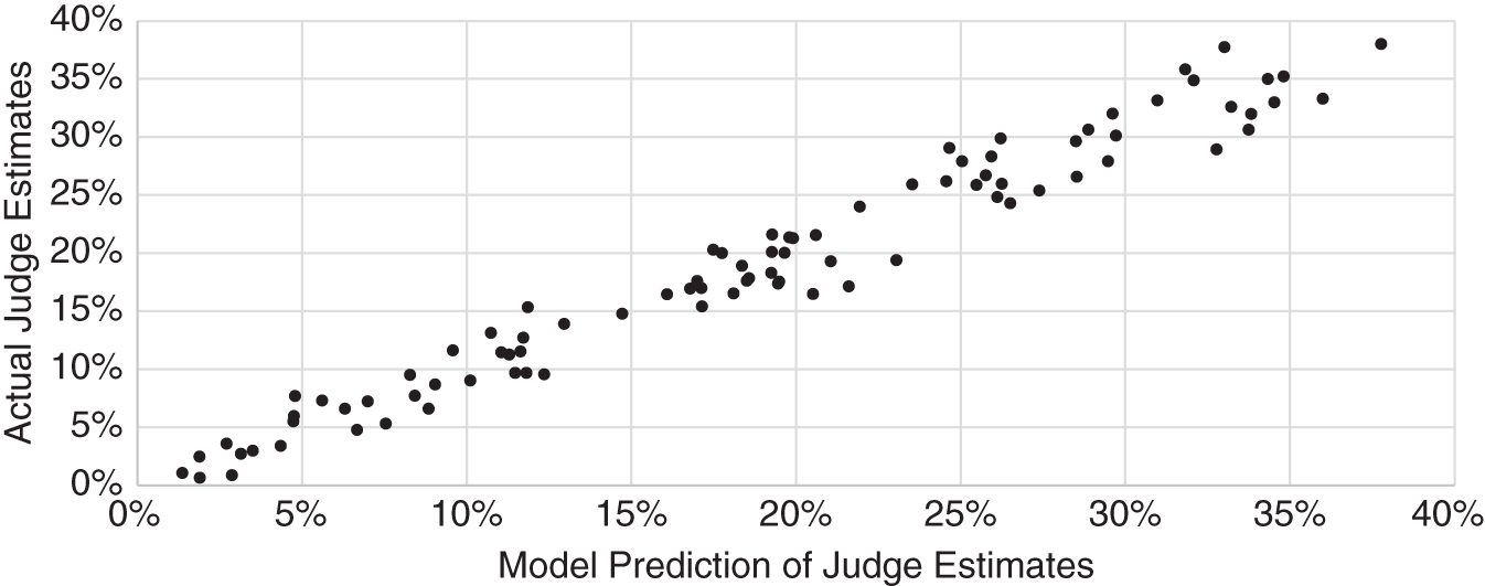
FIGURE 9.5 Example of Regression Model Predicting Judge Estimates
That means the lens model would agree even better if only the experts were more consistent. This inconsistency is eliminated by the lens method. If you decided to tackle the lens method, the model you just produced is actually better than a single expert in several ways. It is actually an emulation of the average of your best calibrated experts if they were perfectly consistent.
To estimate inconsistency we can use the “duplicate pair” method we showed back in Chapter 4 on several conditions instead of asking experts for the effect of individual conditions. For example, the seventh scenario in the list may be identical to the twenty‐ninth scenario in the list. After looking at a couple of dozen scenarios, experts will forget that they already answered the same situation and often will give a slightly different answer. Thoughtful experts are fairly consistent in their evaluation of scenarios. Still, as we showed in Chapter 4, inconsistency accounts for about 21% of the total variation in expert judgments (the remaining 79% due to the data the experts were provided to base their judgments on). This inconsistency is completely removed by the lens method.
Comparing the Lens Method and LOR
There are pros and cons to these two methods of decomposing multiple conditions in an estimate of likelihood:
- LOR takes (a little) less time. The lens method requires experts to answer a large number of samples in order to make it possible to build a regression model.
- The lens method can pick up on more complex interactions between variables. The experts’ responses could indicate that some variables only matter if other variables have a particular value.
- LOR is a bit simpler. The lens method depends on building a regression model that predicts the judgments of experts well. While Excel has tools to simplify this, actually building a good regression often requires several approaches. Perhaps you should make it a nonlinear model by having two variables show a compounding effect. Perhaps you should combine some of the discrete values of a variable (e.g., does “server location” really need to differentiate domestic managed by us, domestic managed by third party, or foreign instead of “we manage it” and “somebody else manages it”?). This is not technically difficult, especially for people who may have the background for this, but it can still be a bit time consuming.
- The LOR tends to give much more variation in estimates than the lens method. The experts will sometimes be surprised how the effects of multiple conditions quickly add up to make an estimated likelihood approaching the extremes of 0 or 1. When the same expert estimates likelihoods in a lens method, they will tend to vary their answers a lot less. Perhaps the expert is underestimating the cumulative effect of independent variables in the LOR method, or perhaps they are being too cautious in modifying their estimates based on the information they are given for the lens method. It will be up to you to decide which is more realistic.
- Both methods help reduce inconsistency, but the lens method provides a more convenient way to measure it. As mentioned earlier, measuring inconsistency is useful because we know that this error is eliminated by the quantitative model and, if we eliminate it, we can estimate how much error was reduced. Since the lens method requires multiple estimates (at least dozens), inconsistency can be easily estimated with the duplicate pair method.
The bottom line is that if you are looking for a quick solution, use the LOR method for decomposing probabilities based on multiple conditions. However, it is important to check how much the answers vary when you change conditions between two extremes (one where all conditions are set to values that increase likelihood, and one where all conditions are set to values that decrease likelihood). If the extremes seem entirely unrealistic, then you might consider reducing the estimates of effects of individual variables, as mentioned earlier.
There is some evidence that people tend to overreact to signals when there are several signals, especially when they are highly correlated. One study calls this a “correlation neglect” when considering conditional probabilities.1 If two signals A and B are perfectly correlated (i.e., if you tell me the value for one, I know exactly the value for the other), then you don't need to know both A and B to estimate some probability X: P(X|A,B) = P(X|A) = P(X|B). However, even when someone is told that A and B are highly correlated, they tend to view them as independent (and therefore reinforcing) signals, and they will overreact when estimating the new conditional probability of X. As we mentioned with LOR earlier, if you suspect two conditions are highly correlated, the simplest fix is to just not use one of them.
Still, even when we use the lens method, we have found it useful to start with LOR just to get the cybersecurity experts to start thinking how knowledge of individual conditions can modify their probabilities. It also helps to eliminate some conditions the experts originally thought might be informative. For example, suppose we are in a workshop and the cybersecurity team is listing conditions they think could be informative for an estimate in a lens model.
One of the participants in a workshop might say they think the type of operating system an asset uses could inform the probability of a breach of the data on that asset. To test this, we employ the LOR process described earlier by asking how much the experts would change the baseline probability (the probability of a cybersecurity event given no information about the asset other than it was one of their own) if they were told that the operating system was Linux and then what they would change it to if they were told the operating system was Microsoft. They might realize that this information would not have caused them to modify the baseline probability. If so, then we can eliminate it from the lens model.
Both the lens and LOR methods raise interesting conceptual obstacles for some experts. They may lack confidence in the process because they have a misunderstanding of how it works. We do not find that most experts we have worked with will have an objection to the process based on one of these misconceptions, but some will. If we know how to address them, then we can help them better understand why their input is needed.
Let's consider the following reaction: “With the lens method, I feel like I am picking answers at random.” If this were the case for most people, we would not see the data that we see. If people estimating probabilities used in the lens method truly were picking values at random, then we would be unable to find correlations that are as strong as we typically find in these models. It would also be a mystery as to why experts—who have plenty of disagreement—actually agree as much as they do.
Clearly, different experts working independently who were picking estimates at random would not agree with each other about how much one condition or another changes the likelihood of an event. And yet we do observe some level of agreement, and the level is far beyond what could be explained by chance. So the expert who has this concern may be expressing that when he or she is faced with individual situations, he or she could have estimated a 5% chance or perhaps 2% or 8%. This is no doubt true. The individual choice seems like you could have estimated a slightly different value and still be satisfied. But, of course, the lens method does not depend on a single estimate or even a single expert. When a large number of data points are brought together, a pattern inevitably forms, even when the experts felt they had some randomness in their responses for individual cases.
We may also hear the reaction, “These variables alone tell me nothing. I need a lot more information to make an estimate.” Whether answering how a single condition can change a probability for a LOR method or answering how estimates changed based on multiple (but still just a few) conditions, some experts will object that without knowing more—indeed, some will say without knowing everything—they cannot provide an estimate. In other words, “Knowing how frequent patches are made will only tell me something about a probability if I also know several other [usually unidentified and endless] things.” This can't be true, and it can be disproven mathematically using the law of total probability.
There is a more formal version of this proof in the original How to Measure Anything, but for now, just know that this position isn't mathematically logical. Another problem with this position is that we know relatively simple models will turn out to be decent predictors of expert judgment. Often, we even end up eliminating one or more variables from a model because they turned out to be unnecessary to predict the expert's judgment. This means that a variable the experts at one point thought was something they considered in their judgments does not appear to have any bearing on their judgment at all. They just discovered what we called in previous chapters an “uninformative decomposition.” We all tend to imagine that our subjective judgments are a result of fairly elaborate and deliberate processing of options. A more realistic description of our judgment is more like a small set of variables in a very simple set of rules added to a lot of noise and error.
As with other methods we mention, you can get some help with LOR and lens with spreadsheets provided at www.howtomeasureanything.com/cybersecurity.
LOR from Other Cyber Professionals
Hubbard and Seiersen have produced several lens models to estimate cybersecurity risks in multiple organizations. When we combine our findings, we can see some simple rules of thumb that you might use in the interim until you have time to build a more complete model.
As the examples above showed, we decomposed the entire organization into some set of subsystems. The subsystems could be critical applications or a broader definition of hundreds or thousands of information assets including specific servers. Or the decomposition could be less granular by defining subsystems as a dozen or so large areas of the network or even departments within the hierarchy of the organization. Usually, though, we see some definition of information asset used as the subsystem.
We can compute a naive probability that a given subsystem, such as an application, would be compromised in the next year. If you believe the chance that your firm—the system—will be breached next year is 10% and you decompose the system into 20 subsystems, we could start with a baseline for each subsystem of 0.5% per year. That is pretty close, but if we wanted to be a bit closer, we would compute the subsystem breach rate per year as
P(subsystem breach per year) = 1 − (1 − P(system breach))^(1/number of subsystems).
In this case we would get 1 − (1 − 0.1)^(1/20) = 0.525%. If you decided on a very granular model with hundreds or thousands of subsystems, you would get a tiny probability per subsystem even if the probability per year of a breach for the system is large.
Then you can start to differentiate those subsystems with the attributes you know about your environment. When we look at all of the lens models we've done so far, we notice some pretty consistent patterns. Our clients identify different predictive attributes to determine the risks, and they estimate the effects of those attributes differently, but there are five attributes that most have identified as relevant and which also have significant effects on their judgement. They are multifactor authentication, encryption, number of users, whether an asset is Internet‐facing, and the physical location of an asset. Table 9.2 shows the LOR adjustments for each of these attributes.
In other words, if we are using this to work out the effects of MFA on the event probability of a given subsystem, MFA will have a LOR of 2.2 less than not having MFA. If a subsystem with MFA had a 1% chance per year of being breached, then a subsystem without MFA would have to have a chance of being breached closer to 8.4%.
We would have to also check this with our law of total probability against naive baseline for a given subsystem based on the overall system probability and the number of subsystems. If 40% of our subsystems had MFA, then we would have to ensure that 0.4 × 0.01 + (1 − 0.4) × 0.084 was equal to our baseline. If not, we may need to modify our baseline, our share of subsystems with MFA, or how much MFA changes the probability of the event. The share of subsystems with that control can usually be measured exactly by auditing the environment, so it may need to stay fixed. You may consider changing how big of a difference the control makes between having that control and not having it, as expressed by the Table 9.2. It is, after all, only based on a small sample of very different firms.
TABLE 9.2 LOR Effect of Five Major Subsystem Attributes and Proportions within the System Based on Client Surveys
| Attribute | Approximate Median LOR Difference from Previous Lens Surveys | Avg. Proportion of Subsystems in Client Data w/Stated Attribute |
|---|---|---|
| Multifactor authentication implemented | −2.2 | 51% |
| Data encrypted | −2.2 | 48% |
| High user count (10,000+ vs. under 100) | +1.5 | 62% |
| Secured/internal physical location vs. external vendor hosted | −1.7 | 70% |
| Internet‐facing | +2.8 | 47% |
Modifying the baseline may make sense if you believe that your use of MFA and other controls was very different than the industry. We provided the average from our clients of the share of subsystems with each attribute in case that has some bearing on how you think your firm compares to industry data.
Once you compute relevant probabilities in your environment, you may notice that the attribute values of the big five make a smaller difference than you would have imagined otherwise. MFA reduces the probability of a successful breach by a lot but not by a factor of 100 as some vendors might claim. Encrypting data has about the same effect. The calibrated SMEs who provided these estimates were simply being realistic. There are a lot of ways even encrypted, MFA‐protected data could still be breached even if only by human error.
We can also model uncertainty around all of this data. Each conditional probability can be modeled with a beta distribution to represent our uncertainty about the effect of each attribute on subsystem risk. You can go to the book website to download a spreadsheet that can help you with checking whether the values you choose are internally consistent.
An LOR for Aggregating Experts
When we discussed calibrating experts in Chapter 7, we mentioned that there are some ways to combine multiple expert estimates that outperform the best individual. Methods which use algorithms to do this depend on putting multiple independent estimates from SMEs into a formula that computes a new value. A simple algorithmic approach is averaging the expert estimates, but we can do better. One of the best approaches uses Bayesian methods to treat additional estimates from SMEs as updates to previous estimates. Usually, we think of using empirical observations for Bayesian updates of priors. But, in a way, additional SME estimates are adding new information because their knowledge is at least somewhat complementary.
Each SME is adding new information to the group as long as two conditions are met. First, their answers are correlated to actual outcomes (e.g., they know something about their field and don't just guess randomly). Second, SMEs’ estimates are not highly correlated to each other. If two SMEs were highly correlated to each other, you could always accurately estimate the second SME's estimate from the first SME's estimate in which case the second person added no information. If SMEs are highly correlated, the best estimate will be closer to the average estimate.
Hubbard Decision Research has a database of hundreds of thousands of estimates from thousands of SMEs who have gone through calibration training, and some of them are tracked in real‐world estimates after training is completed. This provides a lot of data about how to adjust SME estimates and combine them based on how correlated they are, and we can fine‐tune this based on different categories of estimates. HDR uses a hybrid Bayesian method along with some machine learning to find the best algorithms for combining SMEs.
But you can use a quick method for combining just two SMEs. Keeping the number of SMEs this low reduces the problems introduced by SME correlation. So you don't need to try to gather enough data to determine how correlated teams of SMEs may be.
- Produce a list of events to estimate. The more, the better. You may ask for annual breach probabilities for each department, business critical application, vendor, or other asset. Ask for probabilities of various sorts of events and attack vectors, such as ransomware and denial of service.
- Recruit the best two SMEs. They are not only your most knowledgeable but were the best performers in calibration tests.
- Ask each SME to provide a list of probability estimates for each event in the list you provided.
- Convert all the probabilities each SME provided to a “log odds ratio”: ln(p/(1 − p)).
- For each SME, average the LOR of all estimates. This will produce a SME average. We'll call this “SMEAvgL.”
- For each estimate, average the LOR from each SME to produce an event average. This is “EventAvgL.”
- Average all LORs for all events from all SMEs to get global LOR, “GAvg.”
- For each event compute the extreme combined LOR, “ECLOR.”
ECLOR=GAvg + sum(EventAvgL) − sum(SMEAvg).
- Convert this back to an extreme combined probability, ECP and Event Average Probability, EventAvgP.
- Compute ECP = 1/(1 + 1/exp(ECLOR)) and EventAvgP = 1/(1 + 1/exp(EventAvgL)).
- Your combined estimate will be somewhere between the ECP and EventAvgP. If you think the experts are highly correlated, then the final probability of an event will be closer to the event average probability. If you think the SMEs are highly independent thinkers, then the final probability will be closer to the extreme combined probability.
As with many other methods in this book, you can also find a spreadsheet for computing all of these steps by going to www.howtomeasureanything.com/cybersecurity.
Reducing Uncertainty Further and When to Do It
We don't have to rely on calibrated estimates and subjective decompositions alone. Ultimately, we want to inform estimates with empirical data. For example, conditional probabilities can be computed based on historical data. Also, the beta distribution and other methods for computing conditional probabilities can be combined in interesting ways. We can even make rational decisions about when to dive deeper based on the economic value of the information.
Estimating the Value of Information for Cybersecurity: A Very Simple Primer
Hubbard's first book, How to Measure Anything, gets into a lot more detail about how to compute the value of information than we will cover here. But there are some simple rules of thumb that still apply and a procedure we can use in a lot of situations specific to cybersecurity.
Information has value because we make decisions with economic consequences under a state of uncertainty. That is, we have a cost of being wrong and a chance of being wrong. The product of the chance of being wrong and the cost of being wrong is called the expected opportunity loss (EOL). In decision analysis, the value of information is just a reduction in EOL. If we eliminate uncertainty, EOL goes to zero and the difference in EOL is the entire EOL value. We also call this the expected value of perfect information (EVPI). We cannot usually eliminate uncertainty, but the EVPI provides a useful upper limit for what additional information might be worth. If the EVPI is only $100, then it's probably not worth your time for any amount of uncertainty reduction. If the EVPI is $1 million, then reducing uncertainty is a good bet even if you can reduce it only by half for a cost of $20,000 (the cost could simply be your effort in the analysis).
In cybersecurity, the value of information will always be related to decisions you could make to reduce this risk. You will have decisions about whether to implement certain controls, and those controls cost money. If you choose to implement a control, the “cost of being wrong” is spending money that turns out you didn't need to spend on the control. If you reject the control, the cost of being wrong is the cost of experiencing the event the control would have avoided.
TABLE 9.3 Cybersecurity Control Payoff Table
| Event Didn't Occur | Event Occurs | |
|---|---|---|
| Decided to implement the control | The cost of the control | The cost of the control |
| Decided against the control | Zero | The cost of the event |
In www.howtomeasureanything.com/cybersecurity we have also provided a spreadsheet for computing the value of information. Table 9.3 shows how values in the spreadsheet's payoff table would be structured. Note that we've taken a very simple example here by assuming that the proposed control eliminates the possibility of the event. But if we wanted, we could make this a bit more elaborate and consider the possibility that the event still happens (presumably with a reduced likelihood and/or impact) if the control is put in place.
The calculation is simple. Based on the probability of an event, the cost of the control, and the cost of an event without the control, we compute an EOL for each strategy—implementing or not implementing the control. That is, based on the strategy you choose, we simply compute the cost of being wrong and the chance of being wrong for each strategy.
You can try various combinations of conditional probabilities, costs of events, and costs of controls in the spreadsheet. But it still comes down to this: if you reject a control, the value of information could be as high as the chance of the event times the cost of the event. If you accept a control, then the cost of being wrong is the chance the event won't occur times the cost of the control. So the bigger the cost of the control, the bigger the event it is meant to mitigate, and the more uncertainty you have about the event, the higher the value of additional information.
Using Data to Derive Conditional Probabilities
Let's suppose we've built a model, computed information values, and determined that further measurements were needed. Specifically, we determined that we needed to reduce our uncertainty about how some factor in cybersecurity changes the likelihood of some security event. You have gathered some sample data—perhaps within your own firm or perhaps by looking at industry data—and you organized it as shown in Table 9.4. We can call the occurrence of the event Y and the condition you are looking at X. Using this, we can compute the conditional probability P(Y|X) by dividing the number of rows where Y = Yes and X = No by the total number of rows where X = No. That is, P(Y|X) = (count of Y and X)/count of X (as shown in rule 4—the “it depends” rule—in Chapter 8).
This could be a list of servers for each year showing whether some event of interest occurred on that server and, say, whether it was located offshore or perhaps the type of operating system it had. Or perhaps we wanted to estimate the probability of a botnet infestation on a server based on some continuous value such as the amount of traffic a server gets. (One of our guest contributors, Sam Savage, has shown an example of this in Appendix B.)
If you are handy with pivot tables in Excel, you could do this analysis without too much trouble. But we propose an even easier analytical method using the Excel function =countifs(); the countifs() formula counts the rows in a table where a set of conditions are met. If we count the rows where both columns are equal to “1,” we have the number of times both the event and the condition occurred. This is different from “countif()” (without the “s”), which only counts the number in a given range that meet one criterion. Countifs(), on the other hand, can have multiple ranges and multiple criteria. We need both to compute a conditional probability from a set of historical data.
Counting just the number of 1's in the second column gives us all of the situations where the condition applies regardless of whether the security event occurred. So to compute the conditional probability of an event given a condition, P(Event|Condition), in Table 9.4 we use the following calculation:
(Note, where we say “column A” or “column B” insert the range where your data resides in Excel.)
TABLE 9.4 Table of Joint Occurrences of an Event and a Condition
| Defined Security Event Occurred on This Server | A Stated Condition Exists on That Server |
|---|---|
| 1 | 0 |
| 1 | 1 |
| 0 | 0 |
| 0 | 1 |
| 1 | 1 |
| 1 | 1 |
| 0 | 1 |
Now you are empirically estimating a conditional probability. Again, we've provided a spreadsheet on the website to show how to do this. There is quite a lot of interesting analysis you can do with this approach once you get handy with it.
We've already put as many detailed statistical methods into this book as we think most cybersecurity experts would want to deal with—but the reader could go much further if motivated to do so. Instead of loading more methods at this point, let's just paint a picture of where you could go from here if you feel you are mastering the methods discussed so far.
First, we can combine what we've talked about in much more elaborate and informative ways. For example, instead of using calibrated estimates as inputs for the LOR method, we can use conditional probabilities computed from data in this way as inputs. As with LOR before, as long as the conditions are independent, we can add up the conditional probability with a large number of conditions.
We can also leverage the beta distribution with the empirically derived conditional probability using the data in Table 9.4. If we are using simple binary outcomes (Y) and conditions (X), we can think of them as “hits” and “misses.” For example, you could have a data center where you have layers of controls in place from the network on the host: network firewalls, host firewalls, network intrusion prevention systems, and host intrusion prevention. Lots of investments either way. Suppose we define the outcome variable “Y” as “security incident.” This is very general, but it could be malware, hacking, denial of service, and so on. X, of course, represents the “conditions” we just articulated in terms of layers of controls.
If we count 31 cases where Y and X occur together (security event and controls in place) and 52 total cases of X, then we can estimate the conditional probability with the beta distribution using 31 hits and 21 misses, added to your prior. This allows us to think of our data, again, as just a sample of possibilities and not a reflection of the exact proportion. (More specifically to our example case, we can start forecasting what our controls are saying about the probability of having security incidents.) Instead of adding LORs for fixed conditional probabilities, we randomly draw from a beta distribution and compute the LOR on that output. (This will also have the effect of rotating your LEC in a way that increases the chance of extreme losses.)
Think about how handy this can be if you deal with multiple massive data centers that are deployed globally. You would want to have a sense of the probability of incidents in light of controls. It's an easy step then to determine EVPI in relationship to making a potential strategic change in defenses in light of the simple sample data. Again, you have more data than you think!
Once again, we have provided the spreadsheets at www.howtomeasureanything.com/cybersecurity for detailed examples.
Size as a Baseline Source
In the first edition of this book, we referred to some 2015 research about breach rates conducted by Vivosecurity, Inc. using data from the US Department of Health and Human Services Breach Portal website (aka the HHS “Wall of Shame”). The HHS Breach Portal2 shows PHI record breaches of 500 records or more. Combined with publicly available data about the number of employees for each firm and firms not listed in the site, Vivosecurity estimated the rate of data breaches as of 2015 appears to be about a 14% chance per 10,000 employees per year (this is higher than data on major data breaches since it includes breaches as small as 500 records). This was up slightly from about 10% in 2012.
This relationship between size and breach risk continues since that study. Hubbard Decision Research collected data from publicly available lists of reported data breaches and employee count of Fortune 1000 companies. Our data focuses on breaches that made the news, which were always much larger than the 500 record threshold of the HHS website. Consequently, HDR found a much lower breach rate than Vivosecurity, by a factor of 10 or more, but like the Vivosecurity research found, there was still a strong linear relationship between staff count and breach rate.
The cybersecurity data collection firm Advisen has publicly available data that shows there is a direct relationship between revenue and frequency of breaches. In their data, a firm with between $1 million and $10 million in annual revenue will have about a 2% chance per year of what they define as an “event” and a firm with over $1 billion in revenue will probably have multiple events per year. Like the HHS data, Advisen data will probably be counting some smaller events than the HDR data included, and it includes ransomware and other events that are not counted by HHS. Using NAIC data about the average revenue per employee as a function of headcount, the Advisen data implies a much higher chance per year of a data breach event than even the Vivosecurity data did. The Advisen data is more recent and includes more types of events than Vivosecurity.
Using size measured by either headcount or revenue tells us something about the rate of data breaches and other events. The upshot is that if you want to use more recent data and data for smaller and more types of events, you will need to consider methods that allow for multiple events per year. That is the topic of the next part of this chapter.
More Advanced Modeling Considerations
In the beta distribution example, we were uncertain about the true proportion of some population, and we had to estimate it based on a few samples. The simplifying assumption was that each time period was like drawing a marble from an urn. Just as the marble was either red or green, the event either happened or did not happen in a given year. This assumption is not far off the mark when the probabilities are in the single digits or less.
There are cases where we need to consider the possibility that more than one event could happen in a year. The VERIS database, the IRIS report, and Advisen database show there are real cases of the same organization experiencing a data breach twice or more in a single year. Even though the previously described methods allow for only up to one event in a given period, there is already a possibility of multiple events per year when we decomposed the system into a number of subsystems, each of which have a risk of an event independently of the others. While each subsystem could have at most one event in a year, our simple simulations can generate events for multiple subsystems in the system.
Still, there are situations where we may want to simulate the possibility of multiple events in a given year even for a single subsystem. For that, we will introduce some additional tools: the Poisson distribution and the gamma Poisson distribution.
The Poisson Distribution
The Poisson distribution describes situations where more than one thing can occur in a given interval. We can illustrate this by changing the urn example. Instead of randomly drawing marbles from one urn, suppose we start with a number of empty urns and randomly distribute marbles among them. Let's say we have 100 marbles, and each marble is randomly dropped in an urn. Each marble drop is independent of whether a marble was already dropped in the same urn. In this case, we would not get exactly one marble in each of the 100 urns. In fact, if we repeated this experiment, we would find that about 37 urns were empty, on average. This is because some urns, by chance, would have more than one marble. About 18 would have two, about six would have three, and so on.
Likewise, if we say that the average frequency of an event is once per decade, there is a small chance that the event could happen twice in a year. Just think of each year as an urn that receives randomly dropped marbles representing data breaches or ransomware attacks.
The Poisson distribution gives us the probability for how many marbles (an integer value) would end up in an urn or how many events occur in a given period. For simulations in Excel, we had been using inverse probability functions (norm.inv(), beta.inv(), etc.). There is no such inverse probability function for the Poisson distribution in Excel. But we can approximate it very closely by converting a time interval into much smaller intervals. For tiny intervals, like a millionth of a year, the chance of two or more events occurring in one interval is negligible but multiple intervals within a year can experience and event. This allows us to very closely approximate the inverse Poisson probability function by using the binom.inv() function in Excel.
This will produce almost exactly the same output as a Poisson‐distributed inverse probability function when there are several events per year—as long as it is not hundreds or thousands of events per year. (Note, again, that where we refer to rand(), the spreadsheet at www.howtomeasureanything.com/cybersecurity will actually use the HDR PRNG.)
The Gamma Distribution
Now suppose we change the example further so that we don't actually know the ratio of urns to marbles. Not only do we have uncertainty about how many marbles end up in an urn, but that uncertainty is further complicated by having uncertainty about whether there will be 50 marbles distributed among 100 urns or 200 marbles distributed among 100 urns. This has a significant effect on how many urns we estimate would have a larger number of marbles in them or, analogously, how many years will have multiple events.
We could use a beta distribution in the Excel formula above to represent our uncertainty about the frequency of the event. We could account for this uncertainty if “frequency” in the formula above was given as =beta.inv(rand(),alpha,beta). But there is a more mathematically flexible approach. Remember, the beta distribution can only produce a frequency between 0 and 1. Another distribution used in Bayesian methods is the gamma distribution. The gamma distribution can generate any value greater than zero, including values greater than 1. So if we wanted to say that an event has a frequency of 0.6 to 3.5 times per year, a gamma distribution can handle it. It also lends itself to belief updating just like the beta distribution does with hits and misses.
This can also be simulated in Excel, but we will defer that calculation to the downloadable spreadsheet. For now, we will show an example of how the gamma distribution can be used in the R programming language.
Ransomware, Baselines, and Insurance: A Case Example in R
During RSA and Blackhat in 2022, Seiersen held a series of Cyber Superforecasting training sessions. The majority of the attendees were Fortune 1000 level CISOs. Their learning goals ranged from curiosity stemming from our books to more practical matters such as making defensible budgets and board presentations. Our focus was incorporating SME input into predictive cyber models. To make it extremely practical we zeroed in on ransomware with the objective of forecasting the likelihood of experiencing a material event.
We consider a loss that is reported to insurance that is actually paid out or is part of your deductible as material. A material loss such as this is a surprising amount for both insured and insurer. Exceeding a limit is shocking. For the insured (like the CISOs in our training) you are most concerned about the magnitude of limit exceedance. For example, a 20% chance of exceeding a limit of $100M with a 5% chance of exceeding $200M may be insomnia inducing. But a 3% chance of exceeding $100M with a less than 1% chance of exceeding $200M might be acceptable—relatively speaking.
You could invest in more controls and higher limits. If you exceed your limit, you will find it hard to get your cyber policy renewed. The best‐case scenario is that you get a significant rate hike with shrunken limits (aka sub‐limits). For the CISO, getting and maintaining cyber insurance supports their security goals. It provides a defensible rationale for security investments that their peers, particularly CFOs, will understand. Afterall, the CFO (or GC) is the one responsible for acquiring favorable insurance terms—terms they cannot get without evidence of solid security controls.
Seiersen asked the group what they thought the material event rate was. Estimates of the rate of material ransomware attacks for a single company varied from about once in a decade to once in 75 years with an average of once in 38 company‐years. That is, once in 38 companies in one year, or once in one company over 38 years—in other words, there is a 2.6% chance in a given year of a firm experiencing such an event.
Then, the CISOs in the room were asked how many times they experienced a material ransomware loss in the last five years. To the surprise of the CISOs in the room, none raised their hand. With 10 bona fide CISOs in this sample for a five‐year period, that comes to 50 company‐years of CISO material ransomware experience.
This is empirical data, and it would cause us to update the original beliefs about rates of attacks downward. We could also add to this some actual claims data from a cyberinsurance company, like the one Seiersen works for. In the database of Resilience's clients, Seiersen found 200 where they had at least one year of claims data. From those, there were four ransomware claims. Including the previous CISO survey, this gives us four hits and 246 misses out of a sample of 250. Laplace's rule of succession would tell us that the chance that a given firm would experience material ransomware in a given year is about 1.98%.
You may be wondering why we even care about naive beliefs when we already have claims data? The claims data is biased and not voluminous. Material losses are rare. Also, this data is from one insurance provider focused on midsized firms, it excludes some industries, and Resilience may be more selective in its underwriting process. Do we reject that data? No. We want to be resourceful with whichever data we have. The good news is that our CISOs’ naive forecasts and surveys may help make the data less biased—and vice versa.
Figure 9.6 shows the result of combining this data using the gamma distribution. This was developed using some code in the statistical programming language R. The code is shown at the end of this discussion with comments.
The bottommost curve represents our CISOs’ beliefs about material ransomware arrival rates. Let's now consider the two taller curves. The one farthest to the right represents our data. And the slightly narrower curve is the final posterior. The dotted lines represent the 90% credible interval for the posterior. The credible interval simply says that the rate has a 90% chance of being within those two values—given the current data and the model.
Summarizing the Model Output
- We credibly believe there are between 0.8 and 3 material ransomware events in a 100‐year time frame.
- As a probability, our average expectation is that there is a 1.9% chance of experiencing a material ransomware event per year.

FIGURE 9.6 Bayesian Updating for Ransomware
In this example, the beta distribution would give an answer that is fairly close to the gamma distribution because the probability is small. The R code uses a simulation and will have some sampling error. In this situation, the mean of 1.9% is pretty close to what we estimated with the simple LRS, but now you have another tool for those situations where you may want to model much more frequent events.
Now, does 1.9% seem small? Remember, this is a material ransomware event as we have defined it. That is different from merely experiencing ransomware. Also consider that there are thousands of companies around the world that would be subject to this. For example, what does a 1.9% probability mean across the Fortune 1000? And now consider how much real breach news with measurable impacts you actually see regarding ransomware and that specific population.
Ransomware is only one of dozens of perils a company faces. Each peril will have its own baseline probability of occurring given your data and model. Keep in mind that a baseline is just a starting point. After all, you likely have controls in place (or not) that would either mitigate or exacerbate this baseline.
R Code Used in the Example:
Wrapping Up Bayes
These last two chapters were an introduction to some simple and then some slightly more advanced empirical methods using Bayes. By leveraging already developed spreadsheets for some of the more detailed explanations, we covered quite a lot of ground.
We've shown how the use of Bayesian methods and its derivatives allow cybersecurity to update initial calibrated estimates with new information. We've shown how the use of the Bayesian methods can apply to a simple update problem, but we've also shown how much more elaborate methods such as the beta distribution can still be practically employed by using existing features of Excel. We've shown how multiple conditions can be combined using LOR methods and the lens method, and we've shown how LOR and beta can be combined. We've also shown how these same methods can be used to combine the estimates of two calibrated SMEs, and we showed a solution using different methods in R.
You don't have to adopt all of this at once. Take a one‐step‐at‐a‐time approach if necessary, and add new methods as you master them. You have a variety of choices for how you model something and how you leverage new information—all of which are surely better than guessing or using methods without any mathematical foundation. Now, Part III will introduce some additional concepts and discuss practical considerations in rolling out these methods in an organization.
Notes
- 1. Benjamin Enke and Florian Zimmermann, “Correlation Neglect in Belief Formation,” Discussion Paper No. 7372 (Bonn, Germany: Institute for the Study of Labor, 2013), http://ftp.iza.org/dp7372.pdf.
- 2. US Department of Health and Human Services, Office for Civil Rights, Breach Portal, “Breaches Affecting 500 or More Individuals,” accessed March 21, 2016, https://ocrportal.hhs.gov/ocr/breach/breach_report.jsf.