Appendix C
Markov Chains on Countable State Spaces
We review the basic elements of the Markov Chain theory in the case where the state space is countable or finite.
We start by recalling the definition of a Markov chain process (Δ t ) t ≥ 0 with discrete state space ℰ. The state space ℰ may be infinite – such as the set of the non‐negative integers ℕ = {0, 1, …} – or finite as {1, …, d}. Otherwise stated, we assume that ℰ = ℕ. The following definitions can be easily adapted when the state space is finite.
C.1. Definition of a Markov Chain
To define a Markov Chain we need an initial distribution π 0 = {π 0i } so that at time 0, the chain belongs to the i th state with probability π 0i :

It is not restrictive to assume π 0i > 0 (otherwise, state i can be withdrawn from the state space). We need a set of transition probabilities {p(i, j)} such that, for any t ≥ 0,
The transition probabilities obviously satisfy p(i, j) ≥ 0 for all i, j ∈ ℰ, and ∑ j ∈ ℰ p(i, j) for any i ∈ ℰ. The Markov property states that instead of conditioning by [Δ t = i] in the latter probability, we may condition on the entire history without changing the conditional probability:
for any integers i 0, …, i t − 1, i, j in ℰ (provided P[Δ t = i, Δ t − 1 = i t − 1, …, Δ0 = i 0] > 0).
C.2. Transition Probabilities
The matrix

is called the transition matrix of the Markov chain. Matrix powers of ℙ are defined by ℙ2 = ℙℙ =(p
(2)(i, j))
i, j ∈ ℰ
where ![]() .
1
More generally, we define ℙ
n
= (p
(n)(i, j))
i, j ∈ ℰ
recursively, for any non‐negative integer
n
, with by convention
p
(0)(i, j) =
.
1
More generally, we define ℙ
n
= (p
(n)(i, j))
i, j ∈ ℰ
recursively, for any non‐negative integer
n
, with by convention
p
(0)(i, j) = ![]() i = j
and
p
(1)(i, j) = p(i, j). It can be shown that, for any states
i, j
, and any
n ≥ 0,
i = j
and
p
(1)(i, j) = p(i, j). It can be shown that, for any states
i, j
, and any
n ≥ 0,
The Chapman–Kolmogorov equation, for m, n ≥ 0,
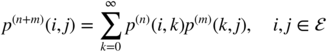
is a consequence of the matrix equality ℙ n + m = ℙ n ℙ m .
C.3. Classification of States
For i, j ∈ ℰ, we say that j is accessible from i , written i → j , if p (n)(i, j) > 0 for some non‐negative integer n . States i and j communicate, written i ↔ j , if i → j and j → i . It can be checked that communication is an equivalence relation. 2
A Markov chain is called irreducible if all states communicate.
The notion of recurrence is related to how often a chain returns to a given state. A state i is called recurrent if, starting from i , the chain returns to i with probability 1 in a finite number of states. More precisely, define the random variable
with τ i = ∞ if the latter set is empty. State i is recurrent if P[τ i < ∞ |Δ0 = i] = 1. On the contrary, state i is called transient if P[τ i = ∞ |Δ0 = i] > 0 (there is a positive probability of never returning to state i ). A state i is called positive recurrent if E[τ i |Δ0 = i] < ∞. The following result is a useful criterion for recurrence/transience (see Resnick 1992, Propositions 2.6.2 and 2.6.3).
It follows that if ℰ is finite, not all states can be transient. 3
States of a Markov chain can also be classified as either periodic or aperiodic. Define the period of state i as
where gcd stands for greatest common divisor. By convention, take d(i) = 1 if the latter set is empty. State i is called aperiodic if d(i) = 1. Otherwise, state i is called periodic with period d(i) > 1.
Recurrence, transience and the period of a state are called solidarity properties of the Markov chain: whenever state i has one of such properties, any state j such that i ↔ j also has the property (see Resnick 1992, Proposition 2.8.1). The Markov chain is called recurrent (resp. aperiodic) if all the states are recurrent (resp. aperiodic).
C.4. Invariant Probability and Stationarity
Let π = {π j , j ∈ ℰ} = (π 0, π 1, …)′ be a probability distribution on the states of the Markov chain. It is called an invariant distribution if
where ℙ′ is the transpose of the transition matrix of the Markov chain. In other words,
If ν = {ν j , j ∈ ℰ} is a sequence of non‐negative constants satisfying ν = ℙ′ ν , call ν an invariant measure. Note that if ∑ j ∈ ℰ ν j = ∞, it is not possible to scale such a measure ν to get an invariant distribution π .
If an invariant probability distribution π exists, and if the initial distribution is such that π 0 = π , then the Markov chain is a stationary process, that is
and any states i 0, …, i k (see Resnick 1992, Proposition 2.12.1).
When the state space ℰ is finite, an invariant distribution π always exists 4 and can be computed by solving C.4.
For infinite state spaces, an invariant distribution π may or may not exist/be unique. We have the following result (see Resnick 1992, Proposition 2.12.3).
C.5. Ergodic Results
By the strong law of large numbers, the empirical mean of a sequence of iid integrable variables converges to the theoretical mean. For stationary and ergodic processes, such a convergence holds in virtue of the ergodic theorem (see Appendix A). For a Markov chain on a countable state space, one may ask whether or not, for some function f : ℰ → ℝ, an empirical mean like

converges when
n → ∞. For instance, if ![]() for
i ∈ ℰ, the empirical mean is the relative frequency that the chain visits state
i
. The following result is a sufficient condition for convergence of such empirical means (see Resnick 1992, Proposition 2.12.4).
for
i ∈ ℰ, the empirical mean is the relative frequency that the chain visits state
i
. The following result is a sufficient condition for convergence of such empirical means (see Resnick 1992, Proposition 2.12.4).
By the dominated convergence theorem, for
f
bounded, it follows that ![]() as
n → ∞. In particular, for
f(k) =
as
n → ∞. In particular, for
f(k) = ![]() {j = k}
we get
{j = k}
we get

under the conditions of Proposition C.3.
C.6. Limit Distributions
A limit distribution is any probability distribution π satisfying
For such a distribution, we have
Thus, when ℰ is finite, ![]() , which shows that
π
is a stationary distribution. In the general case where ℰ is infinite, the limit and the sum cannot be inverted, but the result continues to hold (see Resnick 1992, Proposition 2.13.1).
, which shows that
π
is a stationary distribution. In the general case where ℰ is infinite, the limit and the sum cannot be inverted, but the result continues to hold (see Resnick 1992, Proposition 2.13.1).
The converse of this property requires assumptions on the Markov chain. Under irreducibility and positive recurrence, we only have a Cesro mean limit in (C.5). If, in addition, the chain is aperiodic, we have the following result (see Resnick 1992, Proposition 2.13.2).
A Markov chain which is positive recurrent, aperiodic and irreducible is called ergodic.
C.7. Examples
The example of the Ehrenfest chain (see Exercise 12.6) shows that the existence of a limit distribution may be lost when aperiodicity is relaxed.
The next example shows that, for random walks, recurrence depends on the dimension.
In the following example, the convergence to the limit distribution can be fully characterised.