
CHAPTER 2
Mathematics of Finance
INTEREST RATES
Interest on money borrowed and lent is a feature of our daily lives. Most people have paid and received interest at some point in time. It is a common practice to make investments by buying bonds and debentures, and opening checking, savings, and time deposits with institutions like commercial banks. Bonds and debentures pay interest on their face value or principal. We refer to this as the coupon. Banks, while they do not pay interest on checking accounts, pay interest on savings and time deposits.
In today's consumer-driven economy, it is also a common practice to buy products and services on loan. Borrowing to buy residential property, which is referred to as a mortgage loan, is a major component of the debt taken by individuals and families. People also borrow to fund their academic pursuits in the form of student loans. Retail borrowing to finance various purchases such as automobiles and consumer durables (white goods) is a feature of today's society.
Interest may be construed as the compensation that a lender of capital receives. Why should a lender charge for making a loan? In other words, why not give an interest-free loan? It must be remembered that if you part with your money in order to extend a loan, then you are deprived of an opportunity to use the funds while they are on loan. The interest that you charge is consequently a compensation for this lost opportunity. In economic parlance we would term this as rent. Capital like land and labor are factors of production, and consequently those who seek to use the resources of others must pay a suitable compensation. To give an analogy, take the case of a family that gives its house or apartment to a tenant. It would obviously require the tenant to pay a monthly rent, because as long as he is occupying the property, the owners are deprived of an opportunity to use it themselves. The same principle is applicable in the event of a loan of funds. The difference is that the compensation in the case of property is termed as rent, whereas when it comes to capital, we term it as interest. In the language of economics, both constitute rent, albeit for different resources.
THE REAL RATE OF INTEREST
The price of a factor of production may be set or regulated by the government or may be left to be determined by market forces. In a free market, interest rates on loans are determined by the demand for capital and its supply. One of the key determinants of interest is what is termed as the real rate of interest.
What exactly is the real rate? The real rate may be defined as the rate of interest that would prevail on a riskless investment, in the absence of inflation. What is a riskless investment in practice? A loan to a central or federal government of a country may be termed as riskless, for these institutions are empowered to levy taxes and print money. As a consequence, there is no risk of nonpayment. In the United States, securities such as Treasury bonds, bills, and notes, which are backed by the full faith and credit of the federal government, may therefore be construed as riskless from the standpoint of nonpayment.
Even these Treasury securities, however, are not devoid of risk from the point of view of protection against inflation. What exactly is inflation? Inflation refers to the change in the purchasing power of money, or the change in the price level. Usually inflation is positive, which means that the purchasing power of money will be constantly eroding. There could be less common situations where inflation is negative, a phenomenon that is termed as deflation. In such a situation, the value of a dollar, in terms of the ability to acquire goods and services, will actually increase. We will illustrate our arguments with the help of an example.
Assets such as Treasury securities give us returns in terms of money, without any assurance as to what our ability to acquire goods and services will be at the time of repayment. The rate of return yielded by such securities in dollar terms is termed as the nominal, or the money rate of return. In our illustration the investor got a 10% return on an investment of $1,000. In the situation where the price of a box of chocolates remained at $10, the ability to buy chocolates was enhanced by 10% and consequently the real rate was also 10%. However, when the price of chocolates rose to $12.50 per box, an initial investment of $1,000, which represented an ability to buy 100 boxes of chocolates at the outset, was translated into an ability to buy only 88 boxes at the end of the year. Thus, the real rate of return in this case was negative or was –12% to be precise.
The relationship between the nominal and real rates of return is called the Fisher Hypothesis, after the economist who first postulated it.
THE FISHER EQUATION
Let us consider a hypothetical economy which is characterized by the availability of a single good, namely chocolates. The current price of a box is $P0. Thus, one dollar is adequate to buy 1/P0 boxes of chocolates at today's prices. Let the price of a box after a year be $P1. Assume that while P1 is known with certainty right from the outset, it need not be equal to P0. In other words, although we are allowing for the possibility of inflation, we are assuming that there is no uncertainty regarding the rate of inflation. If the price of a box at the end of the year is P1, one dollar will be adequate to buy 1/P1 boxes after a year.
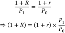
Let us assume that there are two types of bonds that are available to a potential investor. There is a financial bond that will pay $(1 + R) next period per dollar that is invested now, and then there is a goods bond which will return (1 + r) boxes of chocolates next period per box that is invested today. An investment of one dollar in the financial bond will give the investor dollars (1 + R) next period, which will be adequate to buy (1 + R)/P1 boxes. Similarly, an investment of one dollar in the goods bond or 1/P0 boxes in terms of chocolates will yield (1 + r)/P0 boxes after a year.
In order for the economy to be in equilibrium, both the bonds must yield identical returns. Thus, we require that
Inflation is defined as the rate of change in the price level. If we denote inflation by π, then
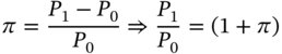
Therefore
This is the Fisher equation. R or the return on the financial bond is the nominal rate of return, while r or the rate of return on the goods bond is the real rate of return. Thus, the relationship is that one plus the nominal interest rate is equal to the product of one plus the real interest rate and one plus the rate of inflation. If the real rate of interest and the rate of inflation are fairly small, then the product ![]() will be of a much smaller order of magnitude. For instance, if r = 0.03 and
will be of a much smaller order of magnitude. For instance, if r = 0.03 and ![]() , then
, then ![]() . If so, we can ignore the product term and rewrite the expression as
. If so, we can ignore the product term and rewrite the expression as
This is called the approximate Fisher relationship.
In Example 2.1, the nominal rate of return was 10% while the rate of inflation was 25%. Thus, the real rate was ![]() .
.
SIMPLE INTEREST & COMPOUND INTEREST
Before analyzing interest computation techniques, let us first define certain key terms.
- Measurement Period: The unit in which time is measured for the purpose of stating the rate of interest is called the measurement period. The most common measurement period is one year, and we will use a year as the unit of measurement unless otherwise specified. That is, we will typically state that the interest rate is x%, say 10%, where the implication is that the rate of interest is 10% per annum.
- Interest Conversion Period: The unit of time over which interest is paid once and is reinvested to earn additional interest is referred to as the interest conversion period. The interest conversion period will typically be less than or equal to the measurement period. For instance, the measurement period may be a year, whereas the interest conversion period may be three months. Thus, interest is compounded every quarter in this case.
- Nominal Rate of Interest: The quoted rate of interest per measurement period is called the nominal rate of interest. For instance, in Example 2.1 the nominal rate of interest is 10%.
- Effective Rate of Interest: The effective rate may be defined as the interest that a dollar invested at the beginning of a measurement period would have earned by the end of the period. Quite obviously the effective rate will be equal to the quoted or nominal rate if the length of the interest conversion period is the same as that of the measurement period, which means that interest is compounded only once per measurement period. However, if the interest conversion period is shorter than the measurement period – or in other words, if interest is compounded more than once per measurement period – then the effective rate will exceed the nominal rate of interest. Take the case where the nominal rate is 10% per annum. If interest is compounded only once per annum, an initial investment of $1 will yield $1.10 at the end of the year, and we would say that the effective rate of interest is 10% per annum. However, if the nominal rate is 10% per annum, but interest is credited every quarter, then the terminal value of an investment of one dollar will definitely be more than $1.10. The relationship between the effective rate and the nominal rate will be derived subsequently. It must be remembered that the term nominal rate of interest is being used in a different context than in the earlier discussion where it was used in the context of the real rate of interest. The potential for confusion is understandable yet unavoidable.
Variables and Corresponding Symbols
- P ≡ amount of principal that is invested at the outset
- N ≡ number of measurement periods for which the investment is being made
- r ≡ nominal rate of interest per measurement period
- i ≡ effective rate of interest per measurement period
- m ≡ number of interest conversion periods per measurement period
Simple Interest
Take the case of an investor who makes an investment of $P for N periods. If interest is paid on a simple basis, then we can state the following.
- The interest that will be earned every period is a constant.
- In every period interest is computed and credited only on the original principal.
- No interest is payable on any interest that has been accumulated at an intermediate stage.
Let r be the quoted rate of interest per measurement period. Consider an investment of $P. It will grow to $P(1 + r) after one period. In the second period, if simple interest is being paid, then interest will be paid only on P and not on P(1 + r). Consequently, the accumulated value after two periods will be $P(1 + 2r). In general, if the investment is made for N periods, the terminal value of the original investment will be $P(1 + rN). N need not be an integer, that is, investments may be made for fractional periods.
Notice the following.
- The interest paid every year is a constant amount of $2,000.
- Every year interest is paid only on the original deposit of $25,000.
- No interest is paid on interest that is accumulated at an earlier stage.
Compound Interest
Let us take the case of an investment of $P that has been made for N measurement periods. However, we will assume this time that interest is compounded at the end of every year. Notice, we are assuming that the interest conversion period is equal to the measurement period, namely a year. In other words, the quoted rate is equal to the effective rate.
In this case, an original investment of $P will become $P(1 + r) dollars after one period. The difference as compared to the earlier case, however, is that during the second period the entire amount will earn interest and consequently the balance at the end of two periods will be P(1 + r)2. Extending the logic the balance after N periods will be P(1 + r)N. Once again you should note that N need not be an integer.
Thus, the following observations are valid if interest is paid on a compound interest basis.
- Every time interest is earned it is automatically reinvested at the same rate for the next conversion period.
- Interest is paid on the accumulated value at the start of the conversion period and not on the original principal.
- The interest earned every period will not be a constant but will steadily increase.
PROPERTIES
- If N = 1, that is, an investment is made for one period, both the simple and compound interest techniques will give the same accumulated value.
In the case of Katherine, the value of her initial investment of $25,000 at the end of the first year was $27,000, irrespective of whether simple or compound interest was used.
- If N < 1, that is, the investment is made for less than a period, the accumulated value using simple interest will be higher. That is
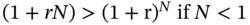
For instance, assume that Katherine deposits $25,000 for nine months at a rate of 8% per annum compounded annually. If interest is calculated on a simple interest basis, she will receive

On the other hand, compound interest would yield

- If N > 1, that is, the investment is made for more than a period, the accumulated value using compound interest will always be greater. That is
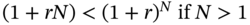
As can be seen, if Katherine were to invest for four years, simple interest will yield $33,000 at the end, whereas compound interest will yield $34,012.2240.
- If the investment is made for one quarter, both simple and compound interest will yield the same terminal value.
- If the investment is made for less than a quarter, the simple interest technique will yield a greater terminal value.
- If the investment is made for more than a quarter, the compound interest technique will yield a greater terminal value.
Simple interest is usually used for short-term or current account transactions, that is, for investments for a period of one year or less. Consequently, simple interest is the norm for money market calculations. The term money market refers to the market for debt securities with a time to maturity at the time of issue of one year or less. In the case of capital market securities, however – that is, medium- to long-term debt securities and equities – we use the compound interest principle. Simple interest is also at times used as an approximation for compound interest over fractional periods.
Effective Versus Nominal Rates of Interest
We will first illustrate the difference between nominal rates and effective rates using a numerical illustration and will then derive a relationship between the two symbolically.
Thus, when the frequencies of compounding are different, comparisons between alternative investments ought to be based on the effective rates of interest and not on the nominal rates. In our case, an investor who is contemplating a deposit of say $10,000 for a year would choose to invest with HSBC despite the fact that its quoted or nominal rate is lower.
A SYMBOLIC DERIVATION
Let us assume that an investor is being offered a nominal rate of r% per annum, and that interest is being compounded m times per annum. In the earlier example, since HSBC was compounding on a monthly basis, m was 12. The effective rate of interest i is therefore given by
We can also derive the equivalent nominal rate if the effective rate is given.
We have already seen how to convert a quoted rate to an effective rate. We will now demonstrate how the rate to be quoted can be derived based on the desired effective rate.
Assume that HSBC Bank wants to offer an effective annual rate of 12% per annum with quarterly compounding. The question is what nominal rate of interest should it quote?
In this case, i = 12%, and m = 4. We have to calculate the corresponding quoted rate r.
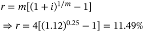
Thus, a quoted rate of 11.49% with quarterly compounding is tantamount to an effective annual rate of 12% per annum. Hence HSBC should quote 11.49% per annum.
PRINCIPLE OF EQUIVALENCY
Two nominal rates of interest compounded at different intervals of time are said to be equivalent if they yield the same effective interest rate for a specified measurement period.
Assume that ING Bank is offering 10% per annum with semiannual compounding. What should be the equivalent rate offered by a competitor, if it intends to compound interest on a quarterly basis?
The first step in comparing two rates that are compounded at different frequencies is to convert them to effective annual rates. The effective rate offered by ING is:
The question is, what is the quoted rate that will yield the same effective rate if quarterly compounding were to be used?
Hence 10% per annum with semiannual compounding is equivalent to 9.88% per annum with quarterly compounding, because in both cases the effective annual rate is the same.
CONTINUOUS COMPOUNDING
We know that if a dollar is invested for N periods at a quoted rate of r% per period and if interest is compounded m times per period, then the terminal value is given by the expression
In the limit as ![]()
where e = 2.71828. Known as the Euler number or Napier's constant, e is defined by the expression:
This limiting case is referred to as continuous compounding. If r is the nominal annual rate, then the effective annual rate with continuous compounding is er − 1.
Continuous compounding is the limit of the compounding process as we go from annual, to semiannual, on to quarterly, monthly, daily, and even shorter intervals. This can be illustrated with the help of an example.
FUTURE VALUE
We have already encountered the concept of future value in our discussion thus far, although we have not invoked the term. What exactly is the meaning of the future value of an investment? When an amount is deposited for a certain time period at a given rate of interest, the amount that is accrued at the end of the designated period of time is called the future value of the original investment.
For instance, if we were to invest $P for N periods at a periodic interest rate of r%, then the future value of the investment is given by
The expression (1 + r)N is the amount to which an investment of $1 will grow at the end of N periods, if it is invested at a rate r. It is called the FVIF (Future Value Interest Factor). It depends only on two variables, namely the periodic interest rate, and the number of periods. The advantage of knowing the FVIF is that we can find the future value of any principal amount, for given values of the interest rate and time period, by simply multiplying the principal by the factor. The process of finding the future value given an initial investment is called compounding.
PRESENT VALUE
Future value calculations entailed the determination of the terminal value of an initial investment. Sometimes, however, we may seek to do the reverse. That is, we may have a terminal value in mind, and seek to calculate the quantum of the initial investment that will result in the desired terminal cash flow, given an interest rate and investment horizon. Thus, in this case, instead of computing the terminal value of a given principal, we seek to compute the principal that corresponds to a given terminal value. The principal amount that is obtained in this fashion is referred to as the present value of the terminal cash flow.
The Mechanics of Present Value Calculation
Take the case of an investor who wishes to have $F after N periods. The periodic interest rate is r%, and interest is compounded once per period. Our objective is to determine the initial investment that will result in the desired terminal cash flow. Quite obviously
where P.V. is the present value of $F.
The expression 1/(1 + r)N is the amount that must be invested today if we are to have $1 at the end of N periods, if the investment were to pay interest at the rate of r% per period. It is called the PVIF (Present Value Interest Factor). It too depends only on two variables, namely the interest rate per period and the number of periods. If we know the PVIF for a given interest rate and time horizon, we can compute the present value of any terminal cash flow by simply multiplying the quantum of the cash flow by the factor. The process of finding the principal corresponding to a given future amount is called discounting and the interest rate that is used is called the discount rate. Quite obviously, there is a relationship between the present value factor and the future value factor, for assumed values of the interest rate and the time horizon. One factor is simply a reciprocal of the other.
HANDLING A SERIES OF CASH FLOWS
Let us assume that we wish to compute the present value or the future value of a series of cash flows, for a given interest rate. The first cash flow will arise after one period, and the last will arise after N periods. In such a situation, we can simply find the present value of each of the component cash flows and add up the terms in order to compute the present value of the entire series. The same holds true for computing the future value of a series of cash flows. Thus present values and future values are additive in nature.
There is a relationship between the present value of the vector of cash flows as a whole and its future value. It may be stated as:
In this case
THE INTERNAL RATE OF RETURN
Consider a deal where we are offered the vector of cash flows depicted in Table 2.4, in return for an initial investment of $30,000. The question is, what is the rate of return that we are being offered? The rate of return r is obviously the solution to the following equation.

The solution to this equation is termed as the Internal Rate of Return. It can be obtained using the IRR function in EXCEL. In this case the solution is 11.6106%.
The present value is higher when we use an effective annual rate of 8% for discounting. This is because the lower the discount rate, the higher will be the present value; obviously, an effective annual rate of 8% is lower than a nominal annual rate of 8% with semiannual compounding. Because the interest rate that is used is lower, the future value at the end of four half-years is lower when we use an effective annual rate of 8%.
In this case, if we were to calculate the IRR for the given cash flow stream, we would get a semiannual rate of return. We would then have to multiply it by two to get the annual rate of return. The IRR for this cash flow stream, assuming an initial investment of $12,500, is 6.2716%. The IRR in annual terms is therefore 12.5432%.
EVALUATING AN INVESTMENT
Kapital Markets is offering an instrument that will pay $25,000 after four years in return for an initial investment of $12,500. Alfred is a potential investor, who requires a rate of return of 12% per annum. The issue is, is the offer attractive from his perspective? There are three ways of approaching this problem.
The Future Value Approach
Let us assume that Alfred buys this instrument for $12,500. If the rate of return received by him were to be 12%, he would have to receive a future value of $19,669. This can be stated as:
If Alfred were to receive a higher terminal payment, his rate of return would be higher than 12%, else it would be lower. Because the instrument offered to him promises a terminal value of $25,000, which is greater than the required future value of $19,669, the investment is attractive from his perspective.
The Present Value Approach
The present value of $25,000 using a discount rate of 12% per annum is:
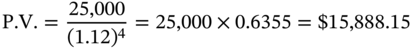
The rate of return, if one were to make an investment of $15,888.15 in return for a payment of $25,000 four years hence, is 12%. If the investor were to pay a lower price at the outset, he would earn a rate of return that is higher than 12%, whereas if he were to invest more, he would obviously earn a lower rate of return. In this case Alfred is being asked to invest $12,500, which is less than $15,288.15. Consequently, the investment is attractive from his perspective.
The Rate of Return Approach
If Alfred were to pay $12,500 in return for a cash flow of $25,000 after four years, his rate of return may be computed as:

Since the actual rate of return obtained by Alfred is greater than the required rate of return of 12%, the investment is attractive.
Not surprisingly, all three approaches lead to the same decision.
ANNUITIES: AN INTRODUCTION
An annuity is a series of payments made at equally spaced intervals of time. If all the payments are identical, then we term it as a Level Annuity. Examples include insurance premiums and monthly installments on housing loans and automobile loans, which are paid off by way of equal installments over a period of time.
If the first payment is made or received at the end of the first period, then we call it an ordinary annuity. Examples include salary, which will be paid only after an employee completes his duties for the month, and house rent, which will be usually paid by the tenant only at the end of the month. The interval between successive payments is called the payment period. We will assume that the payment period is the same as the interest conversion period. That is, if the annuity pays annually, we will assume annual compounding, whereas if it pays semiannually we will assume half-yearly compounding. This assumption is not mandatory and, in practice, we can easily handle cases where the payment period is longer than the interest conversion period, as well as instances where it is shorter.
Consider a level annuity that makes periodic payments of $A for N periods. On a timeline the cash flows can be depicted as shown in Figure 2.1. The point in time at which we are is depicted as time 0.
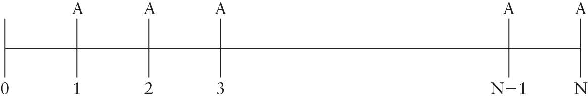
FIGURE 2.1 Timeline for an Annuity
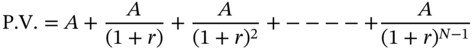
Assume that the applicable interest rate per period is r%. We can then calculate the present and future values as shown here.
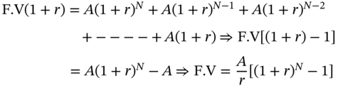
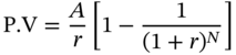
Present Value

Therefore,
 is called the Present Value Interest Factor Annuity (PVIFA). PVIFA(r,N) is the present value of an annuity that pays $1 at periodic intervals for N periods, computed using a discount rate of r%. Thus, like the factors that we studied earlier, it too depends on the interest rate and the number of periods. The present value of any annuity that pays $A per period can therefore be computed by multiplying A by the appropriate value of PVIFA.
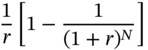
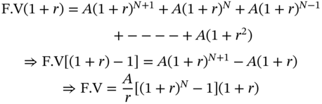
Future Value
Similarly, we can compute the future value of a level annuity that makes N payments, by compounding each cash flow until the end of the last payment period.
Therefore,
![]() is called the Future Value Interest Factor Annuity (FVIFA). This is the future value of an annuity that pays $1 per period for N periods, where interest is compounded at the rate of r% per period. The advantage once again is that if we know the factor, we can calculate the future value of any annuity that pays $A per period.
is called the Future Value Interest Factor Annuity (FVIFA). This is the future value of an annuity that pays $1 per period for N periods, where interest is compounded at the rate of r% per period. The advantage once again is that if we know the factor, we can calculate the future value of any annuity that pays $A per period.
ANNUITY DUE
The difference between an annuity and an annuity due is that in the case of an annuity due the cash flows occur at the beginning of the period. An N period annuity due that makes periodic payments of $A may be depicted as follows

Present Value
Therefore,

The present value of an annuity due that makes N payments is obviously greater than that of a corresponding annuity that makes N payments, because in the case of the annuity due, each of the cash flows has to be discounted for one period less. Consequently, the present value factor for an N period annuity due is greater than that for an N period annuity by a factor of (1 + r).
An obvious example of an annuity due is an insurance policy, because the first premium has to be paid as soon as the policy is purchased.
Future Value
Therefore,
Hence
The future value of an annuity due that makes N payments is higher than that of a corresponding annuity that makes N payments, if the future values in both cases are computed at the end of N periods. This is because, in the first case, each cash flow has to be compounded for one period more.
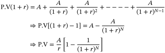
PERPETUITIES
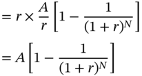
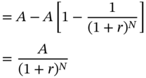
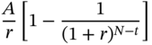
An annuity that pays forever is called a perpetuity. The future value of a perpetuity is obviously infinite. But it turns out that a perpetuity has a finite present value. The present value of an annuity that pays for N periods is
The present value of the perpetuity can be found by letting N tend to infinity. As follows:
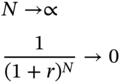
Thus, the present value of a perpetuity is A/r.
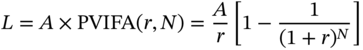
THE AMORTIZATION METHOD
The amortization process refers to the process of repaying a loan by means of regular installment payments at periodic intervals. Each installment includes payment of interest on the principal outstanding at the start of the period and a partial repayment of the outstanding principal itself. In contrast, an ordinary loan entails the payment of interest at periodic intervals, and the repayment of principal in the form of a single lump-sum payment at maturity. In the case of an amortized loan, the installment payments form an annuity whose present value is equal to the original loan amount. An Amortization Schedule is a table that shows the division of each payment into a principal component and an interest component and displays the outstanding loan balance after each payment.
Take the case of a loan which is repaid in N installments of $A each. We will denote the original loan amount by L, and the periodic interest rate by r. Thus this is an annuity with a present value of L, which is repaid in N installments.
The interest component of the first installment
The principal component
The outstanding balance at the end of the first payment
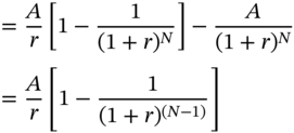
In general, the interest component of the ‘t’th installment is
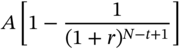
The principal component of the ‘t’th installment is
and the outstanding balance at the end of the ‘t’th payment is
We will analyze the first few entries in Table 2.6 in order to clarify the principles involved. At time 0, the outstanding principal is $25,000. After one period, a payment of $4,350.37 will be made. The interest due for the first period is 8% of $25,000, which is $2,000. Consequently, the excess payment of $2,350.37 represents a partial repayment of principal. Once this amount is repaid and adjusted toward the principal, the outstanding balance at the end of the first period will become $22,649.63. At the end of the second period, the second installment of $4,350.37 will be paid. The interest due for this period is 8% of the outstanding balance at the start of the period, which is $22,649.63. Thus the interest component of the second installment is $1,811.97. The balance, which is $2,538.40, constitutes a partial repayment of principal. The value of the outstanding principal at the end should be zero. As can be seen, the outstanding principal declines after each installment payment. Because the payments themselves are constant, the interest component will steadily decline while the principal component will steadily increase.
TABLE 2.6 An Amortization Schedule
| Year | Payment | Interest | Principal Repayment | Outstanding Principal |
|---|---|---|---|---|
| 0 | 25,000 | |||
| 1 | 4,350.37 | 2,000.00 | 2,350.37 | 22,649.63 |
| 2 | 4,350.37 | 1,811.97 | 2,538.40 | 20,111.23 |
| 3 | 4,350.37 | 1,608.90 | 2,741.47 | 17,369.76 |
| 4 | 4,350.37 | 1,389.58 | 2,960.79 | 14,408.97 |
| 5 | 4,350.37 | 1,152.72 | 3,197.65 | 11,211.32 |
| 6 | 4,350.37 | 896.91 | 3,453.46 | 7,757.86 |
| 7 | 4,350.37 | 620.63 | 3,729.74 | 4,028.12 |
| 8 | 4,350.37 | 322.25 | 4,028.12 | 0.00 |
Thus, in the case of such loans, the initial installments will consist largely of interest payments. As we approach the maturity of the loan, however, the corresponding installments will consist largely of principal repayments.
AMORTIZATION WITH A BALLOON PAYMENT
Julie Tate has taken a loan of $25,000 from First National Bank. The loan requires her to pay in eight equal annual installments along with a terminal payment of $5,000. This terminal payment that has to be made over and above the scheduled installment in year eight is termed as a balloon payment. The interest rate is 8% per annum on the outstanding principal. The annual installment may be calculated as follows.
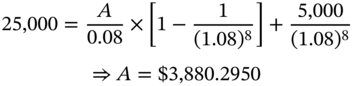
Obviously the larger the balloon, the smaller will be the periodic installment payment for a given loan amount. The amortization schedule may be depicted as shown in Table 2.7.
TABLE 2.7 Amortization with a Balloon Payment
| Year | Payment | Interest | Principal Repayment | Outstanding Principal |
|---|---|---|---|---|
| 0 | 25,000 | |||
| 1 | 3,880.2950 | 2,000.00 | 1,880.30 | 23,119.70 |
| 2 | 3,880.2950 | 1,849.58 | 2,030.72 | 21,088.99 |
| 3 | 3,880.2950 | 1,687.12 | 2,193.18 | 18,895.81 |
| 4 | 3,880.2950 | 1,511.66 | 2,368.63 | 16,527.18 |
| 5 | 3,880.2950 | 1,322.17 | 2,558.12 | 13,969.06 |
| 6 | 3,880.2950 | 1,117.52 | 2,762.77 | 11,206.29 |
| 7 | 3,880.2950 | 896.50 | 2,983.79 | 8,222.50 |
| 8 | 8,880.2950 | 657.80 | 8,222.50 | 0.00 |
THE EQUAL PRINCIPAL REPAYMENT APPROACH
Sometimes a loan may be structured in such a way that the principal is repaid in equal installments. Thus, the principal component of each installment will remain constant; however, as in the case of the amortized loan, the interest component of each payment will steadily decline, on account of the diminishing loan balance. Therefore, the total magnitude of each payment will also decline.
We will illustrate the payment stream for an eight-year loan of $25,000, assuming that the interest rate is 8% per annum (Table 2.8).
TABLE 2.8 Equal Principal Repayment Schedule
| Year | Payment | Interest | Principal Repayment | Outstanding Principal |
|---|---|---|---|---|
| 0 | 25,000 | |||
| 1 | 5,125 | 2,000 | 3,125 | 21,875 |
| 2 | 4,875 | 1,750 | 3.125 | 18,750 |
| 3 | 4,625 | 1,500 | 3,125 | 15,625 |
| 4 | 4,375 | 1,250 | 3,125 | 12,500 |
| 5 | 4,125 | 1,000 | 3,125 | 9,375 |
| 6 | 3,875 | 750 | 3,125 | 6,250 |
| 7 | 3,625 | 500 | 3,125 | 3,125 |
| 8 | 3,375 | 250 | 3,125 | 0.00 |
TYPES OF INTEREST COMPUTATION
Financial institutions employ a variety of techniques to calculate the interest on the loans taken from them by borrowers. Thus the interest rate that is effectively paid by a borrower may be very different from what is being quoted by the lender.1
The Simple Interest Approach
If the lender were to use a simple interest approach, then borrowers need only pay interest for the actual period of time for which they have used the funds. Each time they make a partial repayment of the principal, the interest due will come down for subsequent periods.
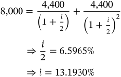
The Add-on Rate Approach
This approach entails the calculation of interest on the entire principal. The sum total of principal and interest is then divided by the number of installments in which the loan is sought to be repaid. As should be obvious, if the loan is repaid in a single annual installment, the total interest payable will be $800 and the effective rate of interest will be 10%. However, if Michael were to repay in two equal semiannual installments of $4,400 each, the effective rate of interest may be computed as follows:
The Discount Technique
In the case of such loans, interest is first computed on the entire loan amount. It is then deducted from the principal, and the balance is lent to the borrower, who has to repay the entire principal at maturity. Such loans are usually repaid in a single installment. Let us take the example of Michael.
The interest for the loan amount of $8,000 is $800. So the lender will give him $7,200 and ask him to repay $8,000 after a year. The effective rate of interest is:
LOANS WITH A COMPENSATING BALANCE
Many banks require borrowers to keep a percentage of the loan amount as a deposit with them. Such deposits, referred to as compensating balances, earn little or no interest. Obviously such requirements will increase the effective rate of interest, and the higher the required balance, the greater will be the rate of interest that is paid by the borrower.
Assume that in Michael's case, the bank required a compensating balance of 12.50%. So while he will have to pay interest on the entire loan amount of $8,000, the usable amount is only $7,000.
The effective rate of interest is:
TIME VALUE OF MONEY–RELATED FUNCTIONS IN EXCEL
We will first demonstrate how to compute effective rates given nominal rates, and vice versa.
The Future Value (FV) Function in Excel
To compute the future value using Excel, we need to use the FV function. The parameters are:
- Rate: Rate is the periodic interest rate.
- Nper: Nper is the number of periods.
- Pmt: Pmt stands for the periodic payment, and is not applicable in this case because there are no periodic cash flows. Thus, we can either put a zero, or an extra comma in lieu.
- Pv: Pv stands for the present value, or the initial investment. We input it with a negative sign in order to ensure that the answer is positive. In many Excel functions, cash flows in one direction are positive while those in the opposite direction are negative. Thus, if the investment is positive, the subsequent inflow is negative, and vice versa. In this case, if we specify a negative number for the present value, we get the future value with a positive sign. If, however, the present value is given with a positive sign, the future value, although it would have the same magnitude, would have a negative sign.
- Type: This is a binary variable, which is either 0 or 1. It is not required at this stage, and we can just leave it blank.
The Present Value Function in Excel
The required function in Excel is PV. The parameters are:
- Rate
- Nper
- Pmt
- Fv
- Type
Fv stands for the future value. The other parameters have the same meaning as specified for the FV function.
COMPUTING THE PRESENT AND FUTURE VALUES OF ANNUITIES AND ANNUITIES DUE IN EXCEL
AMORTIZATION SCHEDULES AND EXCEL
Lorraine has taken a loan of $500,000 which has to be paid back in eight annual installments. The interest rate is 4.80% per annum. The periodic installment can be computed using the PMT function in Excel. The parameters are:
- Rate
- Nper
- PV
- FV
- Type
The values for PV and FV should have opposite signs.
For the first period, ![]()
Now consider the second period. There are two ways in which the PMT function can be invoked. We can specify the same set of parameters as for the first period. Or we can specify the Nper as 7, and the PV as the outstanding balance, which is $447,263.34.
Now consider the interest and principal components of each installment. We can use a function in Excel called IPMT to compute the interest component of an installment and another function called PPMT to compute the principal component of the installment. The parameters, for both, are
- Rate: This is the periodic interest rate.
- Per: This stands for period.
- Nper: This represents the total number of periods.
- Pv: This is the present value.
- Fv: This is the future value.
- Type: This has the usual meaning.
Consider the interest and principal components of the first installment.
![]() . While computing the interest component of the second installment, we can invoke IPMT as IPMT(0.048,2,8,–500000) or as IPMT(0.048,1,7,–447263.94). Both will return a value of $21,468.64. Similarly, the principal component of the first installment is
. While computing the interest component of the second installment, we can invoke IPMT as IPMT(0.048,2,8,–500000) or as IPMT(0.048,1,7,–447263.94). Both will return a value of $21,468.64. Similarly, the principal component of the first installment is ![]() . For the second period,
. For the second period,
IPMT and PPMT can be used with two sets of parameters. We can keep the total number of periods at the initial value, specify the present value as the initial loan amount, and keep changing Per to compute the interest and principal components. For the first installment, Per = 1, and for the nth installment, it is equal to n. The alternative is to re-amortize the outstanding amount at the beginning of each period over the remaining number of periods. Remember that each time we re-amortize, we are back to the first period. Thus, after every payment, we are back to the first period of a loan whose life is equal to the remaining time to maturity, and whose principal amount is equal to the remaining outstanding balance.
NOTE
- 1 To rephrase a famous Microsoft claim, in this case “What You See Is NOT What You Get.”