
Chapter 7
Manipulating Data with Macros
IN THIS CHAPTER
![]() Copying and pasting a range and converting formulas in a range
Copying and pasting a range and converting formulas in a range
![]() Performing text to columns on all columns
Performing text to columns on all columns
![]() Converting trailing minus signs and padding cells with zeros
Converting trailing minus signs and padding cells with zeros
![]() Truncating postal codes to the left five
Truncating postal codes to the left five
![]() Appending text to the left or right of your cells
Appending text to the left or right of your cells
![]() Cleaning up data including duplicates, extra cell space, and blank cells
Cleaning up data including duplicates, extra cell space, and blank cells
![]() Selectively hiding AutoFilter dropdowns
Selectively hiding AutoFilter dropdowns
![]() Copying filtered rows and showing filtered columns in status bar
Copying filtered rows and showing filtered columns in status bar
When working with information in Excel, you often have to transform the data in some way. Transforming it generally means cleaning, standardizing, or shaping data in ways that are appropriate for your work. This can mean anything from cleaning out extra spaces, to padding numbers with zeros, to filtering data for certain criteria.
This chapter shows you some of the more useful macros you can use to dynamically transform the data in your workbooks. If you want, you can combine these macros into one, running each piece of code in a sequence that essentially automates the scrubbing and shaping of your data.
Installing Macros
You can install the macros in this chapter in three places depending on what kind of macro it is and how available you want the macro to be. Event macros are put into the module of the object the event is tied to. Non-event macros go into a standard module and can be in the workbook in which they are meant to run or in a workbook called the Personal Macro Workbook if you want to be able to run them on any workbook.
Event macros
In VBA, objects have events. VBA “listens” for these events to happen and runs special event macros when it detects and event. For example, the workbook object has an Open event. When VBA detects that the workbook has been opened, it looks for a procedure called Workbook_Open in the ThisWorkbook module. If it's there, it runs that macro.
Most of the event macros that you'll use, and most of the examples in the book, are workbook or worksheet events. Workbook event macros go in the ThisWorkbook module and worksheet event macros go in the module for the sheet you want the event code to run on.
To install an event macro, follow these steps:
- Press Alt+F11 to open the VBE.
- In the Project Explorer, find your project/workbook name and click the plus sign next to it to see all the objects.
- Double-click ThisWorkbook.
- Select the event in the right drop-down list.
- Type or paste the code in the module.
Personal Macro Workbook
There is a special workbook called the Personal Macro Workbook named personal.xlsb. If you record a macro, you can choose this workbook as the destination of the recorded macro. The workbook doesn't exist until you first record a macro into it. After that, it lives in a folder and Excel loads that workbook every time it starts.
The benefit of a workbook that opens every time Excel starts is that all the macros in that workbook are always available to you. If you have a macro that works on the active sheet or whatever range is currently selected, that's a good candidate for the Personal Macro Workbook.
To install a macro in the Personal Macro Workbook, follow these steps:
- Press Alt+F11 to open the VBE.
- Right-click personal.xlb in the Project Explorer.
- Choose Insert ⇒ Module.
- Type or paste the code in the newly created module.
 If you don't see personal.xlsb in the Project Explorer, record a macro to the Personal Macro Workbook and Excel will create it for you.
Standard macros
All the other macro examples in this book are installed in a specific workbook in a standard module. If it's not an event macro and it's not a macro you want in the Personal Macro Workbook, then install it using the following steps:
- Press Alt+F11 to open the VBE.
- Right-click the project/workbook name in the Project Explorer.
- Choose Insert ⇒ Module.
- Type or paste the code in the newly created module.
Copying and Pasting a Range
One of the basic data manipulation skills you’ll need is copying and pasting a range of data. It’s fairly easy to do this manually. Luckily, it’s just as easy to copy and paste via VBA.
In this macro, you use the Copy method of the Range object to copy data from D6:D17 and paste it into L6:L17. Note the use of the Destination argument. This argument tells Excel where to paste the data.
Sub CopyAndPasteRange()

  Sheets("Sheet1").Range("D6:D17").Copy _
    Destination:=Sheets("Sheet1").Range("L6:L17")

End Sub
When working with your spreadsheet, you likely often have to copy formulas and paste them as values. To do this in a macro, you can use the PasteSpecial method. In this example, you copy the formulas in F6:F17 to M6:M17. Notice that you’re not only pasting as values using xlPasteValues, but you are also using xlPasteFormats to apply the formatting from the copied range.
Sub CopyAndPasteRange()

  Sheets("Sheet1").Range("F6:F17").Copy
  Sheets("Sheet1").Range("M6:M17").PasteSpecial xlPasteValues
  Sheets("Sheet1").Range("M6:M17").PasteSpecial xlPasteFormats

End Sub
The ranges specified for this macro are for demonstration purposes. Alter the ranges to suit the data in your worksheet.
To implement this macro, you can copy and paste it into a standard module, as outlined in the previous section.
Converting All Formulas in a Range to Values
In some situations, you may want to apply formulas in a certain workbook, but you don’t necessarily want to keep or distribute the formulas with your workbook. In these situations, you may want to convert all the formulas in a given range to values.
In this macro, you use two Range object variables. One of the variables captures the scope of data you’re working with and the other is used to hold each individual cell as you go through the range. Then you use the For Each statement to work with each cell in the target range. In every iteration of the loop, you check to see whether the cell contains a formula. If it does, you replace the formula with the value shown in the cell.
Sub CovertFormulasToValues()

'Step 1: Declare your variables.
  Dim MyRange As Range
  Dim MyCell As Range

'Step 2: Save the workbook before changing cells?
  Select Case MsgBox("Can't undo this action. " & _
        "Save workbook first?", vbYesNoCancel)
    Case vbYes
      ThisWorkbook.Save

    Case vbCancel
      Exit Sub
  End Select

'Step 3: Define the target range.
  Set MyRange = Selection

'Step 4: Start looping through the range.
  For Each MyCell In MyRange

'Step 5: If cell has formula, set to the value shown.
    If MyCell.HasFormula Then
      MyCell.Value = MyCell.Value
    End If

'Step 6: Get the next cell in the range.
  Next MyCell

End Sub
- Declares two Range object variables. One, called MyRange, holds the entire target range. The other, called MyCell, holds each cell in the range as you iterate through the cells one by one.
Shows a message box that gives you three choices: Yes, No, and Cancel. Clicking Yes saves the workbook and continues with the macro. Clicking Cancel exits the procedure without running the macro. Clicking No runs the macro without saving the workbook.
 When you run a macro, it erases the undo stack. This means you can’t undo the changes a macro makes. Because you’re changing data, give yourself the option of saving the workbook before running the macro.
Stores the target range in the MyRange variable, the range that was selected on the spreadsheet in this example.
You can easily set the MyRange variable to a specific range such as Range(“A1:Z100”). Also, if your target range is a named range, you could simply enter its name: Range(“MyNamedRange”).
- Starts looping through each cell in the target range, assigning each cell to the control variable as it loops.
- Checks whether the cell in this iteration contains a formula using the HasFormula property. If it does, the cell's Value property is set equal to itself. This replaces the formula with a hard-coded value.
- Loops back to get the next cell. After all cells in the target range are assigned, the macro ends.
To implement this macro, you can copy and paste it into a standard module, as described in the first section of this chapter, “Installing Macros.”
Text to Columns on All Columns
When you import data from other sources, you may sometimes wind up with cells where the number values are formatted as text. You typically recognize this problem because no matter what you do, you can’t format the numbers in these cells to numeric, currency, or percentage formats. You may also see a smart tag on the cells (see Figure 7-1) that tells you the cell is formatted as text.
It’s easy enough to fix this manually by clicking the Text to Columns command on the Data tab (Figure 7-2). This opens the Text to Columns dialog box shown in Figure 7-3. There is no need to go through all the steps in this wizard; simply click the Finish button to apply the fix.
Again, this is a fairly simple action. The problem, however, is that Excel doesn't let you perform the Text to Columns fix on multiple columns. You have to apply this fix one column at a time. This can be a real nuisance if you have this issue in many columns.
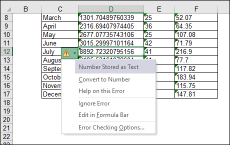
FIGURE 7-1: Imported numbers are sometimes formatted as text.

FIGURE 7-2: Click the Text to Columns command.
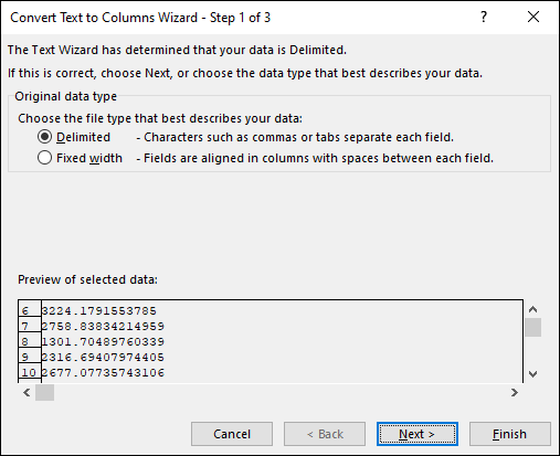
FIGURE 7-3: Clicking Finish in the Text to Columns dialog box corrects incorrectly formatted numbers.
Here is where a simple macro can help you save your sanity. In this macro, you use two Range object variables to go through your target range, using the For Each statement to assign each cell in the target range. Every time a cell is assigned, you reset the value of the cell. This has the same effect as the Text to Columns command.
Sub TTCAllColumns()

'Step 1: Declare your variables.
  Dim MyRange As Range
  Dim MyCell As Range

'Step 2: Save the workbook before changing cells?
  Select Case MsgBox("Can't Undo this action. " & _
            "Save Workbook First?", vbYesNoCancel)
    Case Is = vbYes
      ThisWorkbook.Save

    Case Is = vbCancel
      Exit Sub
  End Select

'Step 3: Define the target range.
  Set MyRange = Selection

'Step 4: Start looping through the range.
  For Each MyCell In MyRange

'Step 5: Reset the cell value.
    If Not IsEmpty(MyCell) Then
      MyCell.Value = MyCell.Value
    End If

'Step 6: Get the next cell in the range.
  Next MyCell

End Sub
- Declares two Range object variables. One, called MyRange, holds the entire target range. The other, called MyCell, holds each cell in the range as you iterate through the cells one by one.
Shows a message box that gives you three choices: Yes, No, and Cancel. Clicking Yes saves the workbook and continues with the macro. Clicking Cancel exits the procedure without running the macro. Clicking No runs the macro without saving the workbook.
Remember that when you run a macro, it erases the undo stack. This means you can’t undo the changes a macro makes. Because you are changing data, give yourself the option of saving the workbook before running the macro.
Stores the target range in the MyRange variable, the range that was selected on the spreadsheet in this example.
You can easily set the MyRange variable to a specific range such as Range(“A1:Z100”). Also, if your target range is a named range, you could simply enter its name: Range(“MyNamedRange”).- Starts looping through each cell in the target range, assigning each cell to the control variable as it loops.
- After a cell is assigned, the IsEmpty function makes sure the cell is not empty. This saves a little time by skipping the cell if there is nothing in it. Then simply set the cell to its own value to force Excel to reevaluate whether the data is numeric.
- Loops back to get the next cell. After all cells in the target range are assigned, the macro ends.
To implement this macro, you can copy and paste it into a standard module. See the earlier section, “Installing Macros,” for the details.
Converting Trailing Minus Signs
Legacy and mainframe systems are notorious for outputting trailing minus signs. In other words, instead of a number such as -142, some systems output 142-. This obviously wreaks havoc on your spreadsheet — especially if you need to perform mathematic operations on the data. This macro goes through a target range and fixes all the negative minus signs so that they show up in front of the number rather than the end.
In this macro, you use two Range object variables to go through your target range, using the For Each statement to assign each cell in the target range. Every time a cell is assigned, you convert the value of the cell into a Double numeric data type by using the Cdbl function. The Double data type forces any negative signs to show at the front of the number.
Sub FixTrailingMinus()

'Step 1: Declare your variables.
  Dim MyRange As Range
  Dim MyCell As Range

'Step 2: Save the workbook before changing cells?
  Select Case MsgBox("Can't Undo this action. " & _
            "Save Workbook First?", vbYesNoCancel)
    Case Is = vbYes
      ThisWorkbook.Save

    Case Is = vbCancel
      Exit Sub
  End Select

'Step 3: Define the target range.
  Set MyRange = Selection

'Step 4: Start looping through the range.
  For Each MyCell In MyRange

'Step 5: Convert the value to a double.
    If IsNumeric(MyCell) Then
      MyCell.Value = CDbl(MyCell.Value)
    End If

'Step 6: Get the next cell in the range.
  Next MyCell

End Sub
- Declares two Range object variables. One, called MyRange, holds the entire target range. The other, called MyCell, holds each cell in the range as you iterate through the cells one by one.
Show a message box that gives you three choices: Yes, No, and Cancel. Clicking Yes saves the workbook and continues with the macro. Clicking Cancel exits the procedure without running the macro. Clicking No runs the macro without saving the workbook.
Remember that when you run a macro, it erases the undo stack. This means you can’t undo the changes a macro makes. Because you are changing data, give yourself the option of saving the workbook before running the macro.
Stores the target range in the MyRange variable, the range that was selected on the spreadsheet in this example.
You can easily set the MyRange variable to a specific range such as Range(“A1:Z100”). Also, if your target range is a named range, you could simply enter its name: Range(“MyNamedRange”).
- Starts looping through each cell in the target range, assigning each cell to the control variable as it loops.
- After a cell is assigned, the IsNumeric function checks whether the value can be evaluated as a number. This is to ensure you don’t affect text fields. Then the cell’s value is passed through the Cdbl function. This converts the value to the Double numeric data type, forcing the minus sign to the front.
Loops back to get the next cell. After all cells in the target range are assigned, the macro ends.
Because you define the target range as the current selection, you want to be sure to select the area where your data exists before running this code. In other words, you wouldn’t want to select the entire worksheet. Otherwise, every empty cell in the spreadsheet would be filled with a zero. Of course, you can ensure this is never a problem by explicitly defining the target range, such as Set MyRange = Range(“A1:Z100”).
To implement this macro, you can copy and paste it into a standard module. The first section in this chapter, “Installing Macros,” details how to do run this macro.
Trimming Spaces from All Cells in a Range
A frequent problem when you import data from other sources is leading or trailing spaces. That is, the imported values have spaces at the beginning or end of the cell. This obviously makes it difficult to do things such as VLOOKUP or sorting. Here is a macro that makes it easy to search for and remove extra spaces in your cells.
In this macro, you enumerate through a target range, passing each cell in that range through the Trim function.
Sub TrimSpaces()

'Step 1: Declare your variables.
  Dim MyRange As Range
  Dim MyCell As Range

'Step 2: Save the workbook before changing cells?
  Select Case MsgBox("Can't Undo this action. " & _
            "Save Workbook First?", vbYesNoCancel)
    Case Is = vbYes
      ThisWorkbook.Save

    Case Is = vbCancel
      Exit Sub
  End Select

'Step 3: Define the target range.
  Set MyRange = Selection

'Step 4: Start looping through the range.
  For Each MyCell In MyRange

'Step 5: Trim the spaces.
    If Not IsEmpty(MyCell) Then
      MyCell = Trim(MyCell)
    End If

'Step 6: Get the next cell in the range.
  Next MyCell

End Sub
- Declares two Range object variables. One, called MyRange, holds the entire target range. The other, called MyCell, holds each cell in the range as you iterate through the cells one by one.
Shows a message box that gives you three choices: Yes, No, and Cancel. Clicking Yes saves the workbook and continues with the macro. Clicking Cancel exits the procedure without running the macro. Clicking No runs the macro without saving the workbook.
Remember that when you run a macro, it erases the undo stack. This means you can’t undo the changes a macro makes. Because you are changing data, give yourself the option of saving the workbook before running the macro.
Stores the target range in the MyRange variable, the range that was selected on the spreadsheet in this example.
You can easily set the MyRange variable to a specific range such as Range(“A1:Z100”). Also, if your target range is a named range, you could simply enter its name: Range(“MyNamedRange”).
- Starts looping through each cell in the target range, assigning each cell to the control variable as it loops.
- After a cell is assigned, the IsEmpty function makes sure the cell is not empty. This saves a little time by skipping the cell if there is nothing in it. The value of that cell passs to the Trim function. The Trim function is a built-in VBA function that removes leading and trailing spaces.
- Loops back to get the next cell. After all cells in the target range are assigned, the macro ends.
Instead of VBA's Trim, you can use Application.WorksheetFunction.Trim to use Excel's TRIM function. Excel's function removes leading and trailing spaces as well as any duplicate spaces within the text.
To implement this macro, you can copy and paste it into a standard module. See the section at the beginning of this chapter, “Installing Macros,” for how to do that.
Truncating Zip Codes to the Left Five
U.S. zip codes are either five or nine digits. Some systems output a nine-digit zip code, which, for the purposes of a lot of Excel analysis, is too many. A common data standardization task is to truncate zip codes to the left five digits. You might use a formula to do this, but if you are constantly cleaning up your zip codes, the macro outlined in this section can help automate that task.
Although this macro solves a specific problem, the concept of truncating data remains useful for many other types of data cleanup activities.
This macro uses the Left function to extract the left five characters of each zip code in the given range.
TruncateZip

'Step 1: Declare your variables.
  Dim MyRange As Range
  Dim MyCell As Range

'Step 2: Save the workbook before changing cells?
  Select Case MsgBox("Can't Undo this action. " & _
            "Save Workbook First?", vbYesNoCancel)
    Case Is = vbYes
      ThisWorkbook.Save

    Case Is = vbCancel
      Exit Sub
  End Select

'Step 3: Define the target range.
  Set MyRange = Selection

'Step 4: Start looping through the range.
  For Each MyCell In MyRange

'Step 5: Extract out the left 5 characters.
    If Not IsEmpty(MyCell) Then
      MyCell = Left(MyCell, 5)
    End If

'Step 6: Get the next cell in the range.
  Next MyCell

End Sub
- Declares two Range object variables. One, called MyRange, holds the entire target range. The other, called MyCell, holds each cell in the range as you iterate through the cells one by one.
Shows a message box that gives you three choices: Yes, No, and Cancel. Clicking Yes saves the workbook and continues with the macro. Clicking Cancel exits the procedure without running the macro. Clicking No runs the macro without saving the workbook.
Remember that when you run a macro, it erases the undo stack. This means you can’t undo the changes a macro makes. Because you’re changing data, give yourself the option of saving the workbook before running the macro.
Stores the target range in the MyRange variable, the range that was selected on the spreadsheet in this example.
You can easily set the MyRange variable to a specific range such as Range(“A1:Z100”). Also, if your target range is a named range, you could simply enter its name: Range(“MyNamedRange”).
- Starts looping through each cell in the target range, assigning each cell to the control variable as it loops.
- After a cell is assigned, the IsEmpty function makes sure the cell is not empty. This saves a little time by skipping the cell if there is nothing in it. The cell’s value passes through the Left function. The Left function allows you to extract out the nth leftmost characters in a string. In this case, you need left five characters to truncate the zip code to five digits.
Loops back to get the next cell. After all cells in the target range are assigned, the macro ends.
As you may have guessed, you can also use the Right function to extract the nth rightmost characters in a string. As an example, it’s not uncommon to work with product numbers where the first few characters hold a particular attribute or meaning, whereas the last few characters point to the actual product (as in 100-4567). You can extract the actual product by using Right(Product_Number, 4). Because the target range is defined as the current selection, you need to select the area where your data exists before running this code. In other words, you wouldn’t want to select cells that don’t conform to the logic you placed in this macro. Otherwise, every cell you select is truncated, whether you mean it to be or not. Of course, you can ensure this is never a problem by explicitly defining the target range, such as Set MyRange = Range(“A1:Z100”).
To implement this macro, you can copy and paste it into a standard module, as outlined in the first section of this chapter, “Installing Macros.”
Padding Cells with Zeros
Many systems require unique identifiers (such as customer number, order number, or product number) to have a fixed character length. For example, you frequently see customer numbers that look like this: 00000045478. This concept of taking a unique identifier and forcing it to have a fixed length is typically referred to as padding. The number is padded with zeros to achieve the prerequisite character length.
It’s a pain to do this manually in Excel. However, with a macro, padding numbers with zeros is a breeze.
Some Excel gurus are quick to point out that you can apply a custom number format to pad numbers with zeros by going to the Format Cells dialog box, selecting Custom on the Number tab, and entering “0000000000” as the custom format.
The problem with this solution is that the padding you get is cosmetic only. A quick glance at the Formula bar reveals that the data actually remains numeric without the padding (it does not become textual). So if you copy and paste the data into another platform or non-Excel table, you lose the cosmetic padding.
If all your customer numbers need to be ten characters long, you need to pad the number with enough zeros to get it to ten characters. This macro does just that.
As you review this macro, keep in mind that you need to change the padding logic in Step 5 to match your situation.
Sub PadWithZeros()

'Step 1: Declare your variables.
  Dim MyRange As Range
  Dim MyCell As Range

'Step 2: Save the workbook before changing cells?
  Select Case MsgBox("Can't Undo this action. " & _
            "Save Workbook First?", vbYesNoCancel)
    Case Is = vbYes
      ThisWorkbook.Save

    Case Is = vbCancel
      Exit Sub
  End Select

'Step 3: Define the target range.
  Set MyRange = Selection

'Step 4: Start looping through the range.
  For Each MyCell In MyRange

'Step 5: Pad with ten zeros then take the right 10.
    If Not IsEmpty(MyCell) Then

      MyCell.NumberFormat = "@"
      MyCell = String(10, "0") & MyCell
      MyCell = Right(MyCell, 10)

    End If

'Step 6: Get the next cell in the range.
  Next MyCell

End Sub
- Declares two Range object variables. One, called MyRange, holds the entire target range. The other, called MyCell, holds each cell in the range as you iterate through the cells one by one.
Shows a message box that gives you three choices: Yes, No, and Cancel. Clicking Yes saves the workbook and continues with the macro. Clicking Cancel exits the procedure without running the macro. Clicking No runs the macro without saving the workbook.
Remember that when you run a macro, it erases the undo stack. This means you can’t undo the changes a macro makes. Because you are changing data, give yourself the option of saving the workbook before running the macro.
Stores the target range in the MyRange variable, the range that was selected on the spreadsheet in this example.
You can easily set the MyRange variable to a specific range such as Range(“A1:Z100”). Also, if your target range is a named range, you could simply enter its name: Range(“MyNamedRange”).
- Starts looping through each cell in the target range, assigning each cell to the control variable as it loops.
After a cell is assigned, the IsEmpty function makes sure the cell isn’t empty. This saves a little time by skipping the cell if there is nothing in it. Ensures the cell is formatted as text so Excel doesn't just drop the leading zeros as soon as you add them by setting the NumberFormat property to the @ symbol. This symbol indicates text formatting.
Concatenates the cell value with ten zeros using the String function, which repeats a character a specified number of times. The ampersand (&) operator concatentates two strings.
The Right function returns the ten rightmost characters. This effectively gives the cell value, padded with enough zeros to make ten characters.
- Loops back to get the next cell. After all cells in the target range are assigned, the macro ends.
To implement this macro, you can copy and paste it into a standard module. See the first section of this chapter, “Installing Macros,” for more information.
Replacing Blanks Cells with a Value
In some analyses, blank cells can cause all kinds of trouble. They can cause sorting issues, they can prevent proper auto filling, they can cause your PivotTables to apply the Count function rather than the Sum function, and so on.
Blanks aren’t always bad, but if they are causing you trouble, you can use this macro to quickly replace the blanks in a given range with a value that indicates a blank cell.
This macro enumerates through the cells in the given range and then uses the Len function to check the length of the value in the assigned cell after it's been trimmed of blank spaces. Trimmed, blank cells have a character length of 0. If the length is indeed 0, the macro enters a 0 in the cell, replacing the blanks. A 0 may not be the appropriate indicator of a blank cell for your specific circumstance, so choose another value if necessary.
Sub ReplaceBlankCells()

'Step 1: Declare your variables.
  Dim MyRange As Range
  Dim MyCell As Range

'Step 2: Save the workbook before changing cells?
  Select Case MsgBox("Can't Undo this action. " & _
            "Save Workbook First?", vbYesNoCancel)
    Case Is = vbYes
      ThisWorkbook.Save

    Case Is = vbCancel
      Exit Sub
  End Select

'Step 3: Define the target range.
  Set MyRange = Selection

'Step 4: Start looping through the range.
  For Each MyCell In MyRange

'Step 5: Ensure the cell has text formatting.
    If Len(Trim(MyCell.Value)) = 0 Then
      MyCell.Value = 0
    End If

'Step 6: Get the next cell in the range.
  Next MyCell

End Sub
- Declares two Range object variables. One, called MyRange, holds the entire target range. The other, called MyCell, holds each cell in the range as you iterate through the cells one by one.
Shows a message box that gives you three choices: Yes, No, and Cancel. Clicking Yes saves the workbook and continues with the macro. Clicking Cancel exits the procedure without running the macro. Clicking No runs the macro without saving the workbook.
Remember that when you run a macro, it erases the undo stack. This means you can’t undo the changes a macro makes. Because you are changing data, give yourself the option of saving the workbook before running the macro.
Stores the target range in the MyRange variable, the range that was selected on the spreadsheet in this example.
You can easily set the MyRange variable to a specific range such as Range(“A1:Z100”). Also, if your target range is a named range, you could simply enter its name: Range(“MyNamedRange”).
- Starts looping through each cell in the target range, assigning each cell to the control variable as it loops.
After a cell is assigned, the Len and Trim functions check whether the value should be replaced.
The Len function is a VBA function that returns a number corresponding to the length of the string being evaluated. If the cell is blank or only contains spaces, the length will be 0; at which point, the macro replaces the cell value with a 0. You could obviously replace the blank with any value you want (N/A, TBD, No Data, and so on).
Loops back to get the next cell. After all cells in the target range are assigned, the macro ends.
Because the target range is defined as the current selection, you want to be sure to select the area where your data exists before running this code. That is to say, you wouldn’t want to select the entire worksheet. Otherwise, every empty cell in the spreadsheet would be filled with a zero. Of course, you can ensure this is never a problem by explicitly defining a range, such as Set MyRange = Range(“A1:Z100”).
To implement this macro, you can copy and paste it into a standard module, as outlined in the first section of this chapter, “Installing Macros.”
Appending Text to the Left or Right of Your Cells
Every so often, you come upon a situation where you need to attach data to the beginning or end of the cells in a range. For example, you may need to add an area code to a set of phone numbers. The macro demonstrates how you can automate the data standardization tasks that require appending data to values.
This macro uses two Range object variables to go through the target range, leveraging the For Each statement to activate each cell in the target range. Every time a cell is activated, the macro attaches an area code to the beginning of the cell value.
Sub AddText()

'Step 1: Declare your variables.
  Dim MyRange As Range
  Dim MyCell As Range

'Step 2: Save the workbook before changing cells?
  Select Case MsgBox("Can't Undo this action. " & _
            "Save Workbook First?", vbYesNoCancel)
    Case Is = vbYes
      ThisWorkbook.Save

    Case Is = vbCancel
      Exit Sub
  End Select

'Step 3: Define the target range.
  Set MyRange = Selection

'Step 4: Start looping through the range.
  For Each MyCell In MyRange

'Step 5: Ensure the cell has text formatting.
    If Not IsEmpty(MyCell.Value) Then
      MyCell.Value = "(972) " & MyCell.Value
    End If

'Step 6: Get the next cell in the range.
  Next MyCell

End Sub
- Declares two Range object variables. One, called MyRange, holds the entire target range. The other, called MyCell, holds each cell in the range as you iterate through the cells one by one.
Shows a message box that gives you three choices: Yes, No, and Cancel. Clicking Yes saves the workbook and continues with the macro. Clicking Cancel exits the procedure without running the macro. Clicking No runs the macro without saving the workbook.
Remember that when you run a macro, it erases the undo stack. This means you can’t undo the changes a macro makes. Because you are changing data, give yourself the option of saving the workbook before running the macro
Stores the target range in the MyRange variable, the range that was selected on the spreadsheet in this example.
You can easily set the MyRange variable to a specific range such as Range(“A1:Z100”). Also, if your target range is a named range, you could simply enter its name: Range(“MyNamedRange”).
- Starts looping through each cell in the target range, assigning each cell to the control variable as it loops.
- After a cell is assigned, ampersand (&) combine an area code with the cell value. If you need to append text to the end of the cell value, you would simply place the ampersand and the text at the end. For example, MyCell.Value = MyCell.Value & “Added Text”.
- Loops back to get the next cell. After all cells in the target range are assigned, the macro ends.
To implement this macro, you can copy and paste it into a standard module. See the earlier section, “Installing Macros,” in this chapter for more details.
Cleaning Up Non-Printing Characters
Sometimes your data includes non-printing characters, such as line feeds, carriage returns, and non-breaking spaces. These characters often need to be removed before you can use the data for serious analysis.
Now, anyone who has worked with Excel for more than a month knows about the Find and Replace function. You may have even recorded a macro while performing a Find and Replace (a recorded macro is an excellent way to automate your find and replace procedures). So your initial reaction may be to simply find and replace these characters. The problem is that these non-printing characters are for the most part invisible and thus difficult to clean up with the normal Find and Replace routines. The easiest way to clean them up is through VBA.
If you find yourself struggling with those pesky invisible characters, use this general-purpose macro to find and remove all the non-printing characters.
This macro is a relatively simple Find and Replace routine. You are using the Replace method, telling Excel what to find and what to replace it with. This is similar to the syntax you would see when recording a macro while manually performing a Find and Replace.
The difference is that instead of hard-coding the text to find, this macro uses character codes to specify your search text.
Every character has an underlying ASCII code, similar to a serial number. For example, the lowercase letter a has an ASCII code of 97. The lowercase letter c has an ASCII code of 99. Likewise, invisible characters also have a code:
- The line feed character code is 10.
- The carriage return character code is 13.
- The non-breaking space character code is 160.
This macro uses the Replace method, passing each character’s ASCII code as the search item. Each character code is then replaced with an empty string:
Sub CleanCells()

'Step 1: Remove line feeds.
  ActiveSheet.UsedRange.Replace What:=Chr(10), Replacement:=""

'Step 2: Remove carriage returns.
  ActiveSheet.UsedRange.Replace What:=Chr(13), Replacement:=""

'Step 3: Remove non-breaking spaces.
  ActiveSheet.UsedRange.Replace What:=Chr(160), Replacement:=""

End Sub
Looks for and removes the line feed character. The code for this character is 10. You can identify the code 10 character by passing it through the Chr function. After Chr(10) is identified as the search item, an empty string is passed to the Replacement argument.
Note the use of ActiveSheet.UsedRange. This tells Excel to look in all the cells that have had data entered into them. You can replace the UsedRange object with an actual range if needed.
- Finds and removes the carriage return character.
- Finds and removes the non-breaking spaces character.
The characters covered in this macro are only a few of many non-printing characters. However, these are the ones you most commonly run into. If you work with others, you can simply add a new line of code, specifying the appropriate character code. You can enter “ASCII Code Listing” in any search engine to see a list of the codes for various characters.
To implement this macro, you can copy and paste it into a standard module, as outlined in the first section of this chapter, “Installing Macros.”
Highlighting Duplicates in a Range of Data
Ever wanted to expose the duplicate values in a range? The macro in this section does just that. There are many manual ways to find and highlight duplicates — ways involving formulas, conditional formatting, sorting, and so on. However, all these manual methods take setup and some level of maintenance as the data changes.
This macro simplifies the task, allowing you to find and highlight duplicates in your data with a click of the mouse (see Figure 7-4).
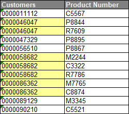
FIGURE 7-4: This macro dynamically finds and highlights the duplicate values in a selected range.
This macro enumerates through the cells in the target range, leveraging the For Each statement to activate each cell one at a time. It then uses the CountIf function to count the number of times the value in the active cell occurs in the range selected. If that number is greater than 1, it formats the cell yellow.
Sub HighlightDupes()

'Step 1: Declare your variables.
  Dim MyRange As Range
  Dim MyCell As Range

'Step 2: Define the target range.
  Set MyRange = Selection

'Step 3: Start looping through the range.
  For Each MyCell In MyRange

'Step 4: Color the cell if there's a duplicate.
    If WorksheetFunction.CountIf(MyRange, MyCell.Value) > 1 Then
      MyCell.Interior.Color = vbYellow
    End If

'Step 5: Get the next cell in the range.
  Next MyCell

End Sub
- Declares two Range object variables. One, called MyRange, holds the entire target range. The other, called MyCell, holds each cell in the range as you iterate through the cells one-by-one.
Stores the target range in the MyRange variable, the range that was selected on the spreadsheet in this example.
You can easily set the MyRange variable to a specific range such as Range(“A1:Z100”). Also, if your target range is a named range, you could simply enter its name: Range(“MyNamedRange”).
- Starts looping through each cell in the target range, assigning each cell to the control variable as it loops.
The WorksheetFunction object provides a way to run many of Excel’s spreadsheet functions in VBA. The WorksheetFunction object runs a CountIf function in VBA.
In this case, you’re counting the number of times the assigned cell value (MyCell.Value) is found in the given range (MyRange). If the CountIf expression evaluates to greater than 1, the macro changes the interior color of the cell.
- Loops back to get the next cell. After all cells in the target range are assigned, the macro ends.
To implement this macro, you can copy and paste it into a standard module. The first section in this chapter, “Installing Macros” has more information.
Hiding All but Rows Containing Duplicate Data
With the previous macro, you can quickly find and highlight duplicates in your data. This in itself can be quite useful. But if you have many records in your range, you may want to take the extra step of hiding all the non-duplicate rows.
Take the example in Figure 7-5. Note that only the rows that contain duplicate values are visible. This more readily exposes the duplicate values because they are the only rows showing.
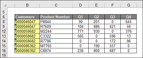
FIGURE 7-5: This macro ensures that only those rows that contain duplicate values are visible.
This macro enumerates through the cells in the target range, leveraging the For Each statement to activate each cell one at a time. It then uses the CountIf function to count the number of times the value in the active cell occurs in the range selected. If that number is 1, it hides the row in which the active cell resides. If that number is greater than 1, it formats the cell yellow and leaves the row visible.
Sub HighlightAndShowDupes()

'Step 1: Declare your variables.
  Dim MyRange As Range
  Dim MyCell As Range

'Step 2: Define the target range.
  Set MyRange = Selection

'Step 3: Start looping through the range.
  For Each MyCell In MyRange

'Step 4: Color the cell if there's a duplicate.
    If Not IsEmpty(MyCell.Value) Then

      If WorksheetFunction.CountIf(MyRange, MyCell.Value) > 1 Then
        MyCell.Interior.Color = vbYellow
        MyCell.EntireRow.Hidden = False
      Else
        MyCell.EntireRow.Hidden = True
      End If

    End If

'Step 5: Get the next cell in the range.
  Next MyCell

End Sub
- Declares two Range object variables. One, called MyRange, holds the entire target range. The other, called MyCell, holds each cell in the range as you iterate through the cells one by one.
Stores the target range in the MyRange variable, the range that was selected on the spreadsheet in this example.
You can easily set the MyRange variable to a specific range such as Range(“A1:Z100”). Also, if your target range is a named range, you could simply enter its name: Range(“MyNamedRange”).
- Starts looping through each cell in the target range, assigning each cell to the control variable as it loops.
The IsEmpty function makes sure the cell is not empty. Do this so the macro won’t automatically hide rows with no data in the target range.
The WorksheetFunction object runs a CountIf function in VBA. This particular scenario counts the number of times the active cell value (MyCell.Value) is found in the given range (MyRange).
If the CountIf expression evaluates to greater than 1, the interior color of the cell is changed and the EntireRow.Hidden property is set to False. This ensures the row is visible.
If the CountIf expression does not evaluate to greater than 1, the macro jumps to the Else argument. Here the EntireRow.Hidden property is set to True. This ensures the row is not visible.
Loops back to get the next cell. After all cells in the target range are assigned, the macro ends.
Because the target range is defined as the current selection, you want to be sure to select the area where your data exists before running this code. You wouldn’t want to select an entire column or the entire worksheet. Otherwise, any cell that contains data that is unique (not duplicated) triggers the hiding of the row. Alternatively, you can explicitly define the target range to ensure this is never a problem — such as Set MyRange = Range(“A1:Z100”).
To implement this macro, you can copy and paste it into a standard module, as shown in the first section of this chapter, “Installing Macros.”
Selectively Hiding AutoFilter Drop-down Arrows
It goes without saying that the AutoFilter function in Excel is one of the most useful. Nothing else allows for faster on-the-spot filtering and analysis. The only problem is that the standard AutoFilter functionality applies drop-down arrows to every column in the chosen dataset (see Figure 7-6). This is all right in most situations, but what if you want to prevent your users from using the AutoFilter drop-down arrows on some of the columns in your data?
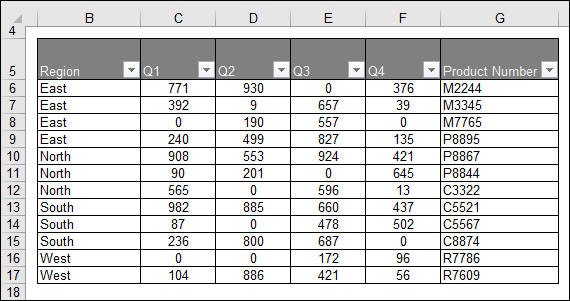
FIGURE 7-6: The standard AutoFilter functionality adds drop-down arrows to all the columns in your data.
The good news is that with a little VBA, you can selectively hide AutoFilter drop-down arrows, as shown in Figure 7-7.

FIGURE 7-7: With a little VBA, you can choose to hide certain AutoFilter drop-down arrows.
In VBA, you can use the AutoFilter object to turn on AutoFilters for a specific range. For example:
Range("B5:G5").AutoFilter
After an AutoFilter is applied, you can manipulate each of the columns in the AutoFilter by pointing to it. For example, you can perform some action on the third column in the AutoFilter, like this:
Range("B5:G5").AutoFilter Field:3
You can perform many actions on an AutoFilter field. In this scenario, you are interested in making the drop-down arrow on field 3 invisible. For this, you can use the VisibleDropDown parameter. Setting this parameter to False makes the drop-down arrow invisible:
Range("B5:G5").AutoFilter Field:3, VisibleDropDown:=False
Here is an example of a macro where you turn on AutoFilters, and then make only the first and last drop-down arrows visible:
Sub HideAutoFilterArrows()

  With Range("B5:G5")
    .AutoFilter
    .AutoFilter Field:=1, VisibleDropDown:=True
    .AutoFilter Field:=2, VisibleDropDown:=False
    .AutoFilter Field:=3, VisibleDropDown:=False
    .AutoFilter Field:=4, VisibleDropDown:=False
    .AutoFilter Field:=5, VisibleDropDown:=False
    .AutoFilter Field:=6, VisibleDropDown:=True
  End With

End Sub
Not only are you pointing to a specific range, but you are also explicitly pointing to each field. When implementing this type of macro in your environment, alter the code to suit your particular data set.
To implement this macro, you can copy and paste it into a standard module. See the first section in this chapter, “Installing Macros,” for more information.
Copying Filtered Rows to a New Workbook
Often, when you're working with an AutoFiltered set of data, you want to extract the filtered rows to a new workbook. Of course, you can manually copy the filtered rows, open a new workbook, paste the rows, and then format the newly pasted data so that all the columns fit. But if you are doing this frequently enough, you may want to have a macro to speed up the process.
This macro captures the AutoFilter range, opens a new workbook, and then pastes the data.
Sub CopyFilteredRows()

'Step 1: Check for AutoFilter — exit if none exists.
  If ActiveSheet.AutoFilterMode = False Then
    Exit Sub
  End If

'Step 2: Copy the AutoFiltered Range to new workbook.
  ActiveSheet.AutoFilter.Range.Copy
  Workbooks.Add.Worksheets(1).Paste

'Step 3: Size the columns to fit.
  Cells.EntireColumn.AutoFit

End Sub
- The AutoFilterMode property checks whether the sheet even has AutoFilters applied. If not, the procedure ends.
- Each AutoFilter object has a Range property. This Range property returns the rows to which the AutoFilter applies, meaning it returns only the rows shown in the filtered data set. The Copy method captures those rows, and then pastes the rows to a new workbook. Workbooks.Add.Worksheets(1) pastes the data into the first sheet of the newly created workbook.
- Adjusts the column widths to autofit the data you just pasted.
To implement this macro, you can copy and paste it into a standard module. See the first section of this chapter, “Installing Macros,” for details.
Showing Filtered Columns in the Status Bar
When you have a large table with many AutoFiltered columns, sometimes it’s hard to tell which columns are filtered and which aren’t. Of course, you could scroll through the columns, peering at each AutoFilter drop-down list for the telltale icon indicating the column is filtered, but that can get old quickly.
This macro helps by specifically listing all the filtered columns in the status bar. The status bar is the bar (shown in Figure 7-8) that runs across the bottom of the Excel window, below the sheet tabs.
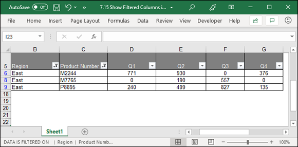
FIGURE 7-8: This macro lists all filtered columns in the status bar.
This macro loops through the fields in your AutoFiltered data set. As it loops, it checks to see whether each field is actually filtered. If so, it captures the field name in a text string. After looping through all the fields, it passes the final string to the StatusBar property.
Sub FilterInStatus()

'Step 1: Declare your variables.
  Dim AF As AutoFilter
  Dim TargetField As String
  Dim sOutput As String
  Dim i As Integer


'Step 2: Check if AutoFilter exists — if not exit.
  If ActiveSheet.AutoFilterMode = False Then
    Application.StatusBar = False
    Exit Sub
  End If

'Step 3: Set AutoFilter and start looping.
  Set AF = ActiveSheet.AutoFilter
  For i = 1 To AF.Filters.Count

'Step 4: Capture filtered field names.
    If AF.Filters(i).On Then
      TargetField = AF.Range.Cells(1, i).Value
      strOutput = sOutput & " | " & TargetField
     End If
  Next i


'Step 5: Display the filters if there are any.
  If Len(sOutput) = 0 Then
    Application.StatusBar = False
  Else
    Application.StatusBar = vbNullString
    Application.StatusBar = "DATA IS FILTERED ON " & sOutput
  End If

End Sub
- Declares four variables. AF is an AutoFilter variable used to manipulate the AutoFilter object. TargetField is a string variable you use to hold the field names of any field that is filtered. The sOutput variable is a string variable used to build out the final text that goes into the status bar. Finally, the i variable serves as a simple counter, allowing you to iterate through the fields in your AutoFilter.
- Checks the AutoFilterMode property to see whether a sheet even has AutoFilters applied. If not, the StatusBar property is set to False. This has the effect of clearing the Status bar and releasing control back to Excel. Then exit the procedure.
- Sets the AF variable to the AutoFilter on the active sheet. The counter starts looping from 1 to the number of columns in the AutoFiltered range. The AutoFilter object keeps track of its columns with index numbers. Column 1 is index 1, column 2 is index 2, and so on. You can loop through each column in the AutoFilter by using the i variable as the index number.
Checks the status of the AF.Filters object for each filter. Pass the i variable to the Filters property to access the filter. If the AutoFilter for that column is filtered in any way, the On property is set to True.
If the filter for the column is on, the value of the header cell is captured in the TargetField variable. Use the Range property of the AF AutoFilter object to get to the whole range. Then use the Cells property to access only the cell for the iteration you're on. Cells(1,1) captures the value in row 1, column 1. Cells(1,2) captures the value in row 1, column 2, and so on.
The row argument to Cells is hard-coded to 1 and the column argument uses the i variable. As the macro iterates through the columns, it always captures the value in the first row of the auto-filtered table as the TargetField name (the first row is where the field name is).
The TargetField name is joined to the sOutput variable with a pipe character to separate multiple fields. The sOutput variable keeps growing as field names are found and tacked on to the end of it.
Checks to make sure that the sOutput string holds a value. If sOutput is empty, it means the macro found no columns in your AutoFilter that were filtered. In this case, s the StatusBar property is set to False, releasing control back to Excel.
If sOutput is not empty, the StatusBar property is set to equal some helper text along with the sOutput string.
You ideally want this macro to run each time a field is filtered. However, Excel does not have an OnAutoFilter event. The closest thing to that is the Worksheet_Calculate event. That being said, AutoFilters in themselves don’t actually calculate anything, so you need to enter a “volatile” function on the sheet that contains your AutoFiltered data. A volatile function is one that forces a recalculation when any change is made on the worksheet.
In the sample files that come with this book, notice that the =Now() function is used. The Now function is a volatile function that returns a date and time. With this on the sheet, the worksheet is sure to recalculate each time the AutoFilter is changed.
Place the Now function anywhere on your sheet (by typing =Now() in any cell). Then copy and paste the macro into the Worksheet_Calculate event Code pane, as shown in Figure 7-9. (See the earlier section, “Installing Macros”, for details.)
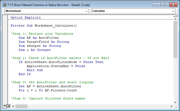
FIGURE 7-9: Type or paste your code in the Worksheet_Calculate event Code pane.
To make the code run as smoothly as possible, consider adding these two pieces of code under the Worksheet_Calculate event:
Private Sub Worksheet_Deactivate()

  Application.StatusBar = False

End Sub

Private Sub Worksheet_Activate()

  Worksheet_Calculate

End Sub
Also, add this piece of code in the workbook BeforeClose event:
Private Sub Workbook_BeforeClose(Cancel As Boolean)

  Application.StatusBar = False

End Sub
The Worksheet_Deactivate event clears the status bar when you move to another sheet or workbook. This avoids confusion as you move between sheets.
The Worksheet_Activate event runs the macro in Worksheet_Calculate. This brings back the status bar indicators when you navigate back to the filtered sheet.
The Workbook_BeforeClose event clears the status bar when you close the workbook. This avoids confusion as you move between workbooks.