
Chapter 5
Working with Worksheets
IN THIS CHAPTER
![]() Adding, naming, copying, and deleting worksheets
Adding, naming, copying, and deleting worksheets
![]() Hiding and unhiding, moving, sorting, and grouping worksheets
Hiding and unhiding, moving, sorting, and grouping worksheets
![]() Protecting and unprotecting all worksheets
Protecting and unprotecting all worksheets
![]() Printing and creating a table of contents for your worksheets
Printing and creating a table of contents for your worksheets
![]() Zooming in and out of a worksheet
Zooming in and out of a worksheet
Excel analysts often need to automate tasks related to worksheets. Whether it is unhiding all sheets in a workbook, or printing all sheets at the same time, many tasks can be automated to save time and gain efficiencies. This chapter covers some of the more useful macros related to worksheets.
Installing Macros
You can install the macros in this chapter in three places depending on what kind of macro it is and how available you want the macro to be. Event macros are put into the module of the object the event is tied to. Non-event macros go into a standard module and can be in the workbook in which they are meant to run or in a workbook called the Personal Macro Workbook if you want to be able to run them on any workbook.
Event macros
In VBA, objects have events. VBA “listens” for these events to happen and runs special event macros when it detects and event. For example, the workbook object has an Open event. When VBA detects that the workbook has been opened, it looks for a procedure called Workbook_Open in the ThisWorkbook module. If it's there, it runs that macro.
Most of the event macros that you'll use, and most of the examples in the book, are workbook or worksheet events. Workbook event macros go in the ThisWorkbook module and worksheet event macros go in the module for the sheet you want the event code to run on.
To install an event macro, follow these steps:
- Press Alt+F11 to open the VBE.
- In the Project Explorer, find your project/workbook name and click the plus sign next to it to see all the objects.
- Double-click ThisWorkbook.
- Select the event in the right drop-down list.
- Type or paste the code in the module.
Personal Macro Workbook
There is a special workbook called the Personal Macro Workbook named personal.xlsb. If you record a macro, you can choose this workbook as the destination of the recorded macro. The workbook doesn't exist until you first record a macro into it. After that, it lives in a folder and Excel loads that workbook every time it starts.
The benefit of a workbook that opens every time Excel starts is that all the macros in that workbook are always available to you. If you have a macro that works on the active sheet or whatever range is currently selected, that's a good candidate for the Personal Macro Workbook.
To install a macro in the Personal Macro Workbook, follow these steps:
- Press Alt+F11 to open the VBE.
- Right-click personal.xlb in the Project Explorer.
- Choose Insert ⇒ Module.
- Type or paste the code in the newly created module.
 If you don't see personal.xlsb in the Project Explorer, record a macro to the Personal Macro Workbook and Excel will create it for you.
Standard macros
All the other macro examples in this book are installed in a specific workbook in a standard module. If it's not an event macro and it's not a macro you want in the Personal Macro Workbook, then install it using the following steps:
- Press Alt+F11 to open the VBE.
- Right-click the project/workbook name in the Project Explorer.
- Choose Insert ⇒ Module.
- Type or paste the code in the newly created module.
Adding and Naming a New Worksheet
This chapter starts with one of the simplest worksheet-related automations you can apply with a macro — adding and naming a new worksheet.
If you read through the lines of the code, you'll see this macro is relatively intuitive.
Sub AddAndNameWorksheet()

'Step 1: Tell Excel what to do if error.
  On Error GoTo MyError


'Step 2: Add a sheet and name it.
  Sheets.Add
  ActiveSheet.Name = _
    Format(Now(), "yyyy_mm:dd_hh_mm:ss")
  Exit Sub


'Step 3: If here, an error happened; tell the user.
MyError:
  MsgBox "There is already a sheet called that."

End Sub
- An error occurs if a sheet is given a name that already exists. Excel skips to the line that says MyError (in Step 3) if there is an error.
The Add method adds a new sheet. By default, the sheet is called Sheetxx, where xx represents the number of the sheet. Give the sheet a new name by changing the Name property of the ActiveSheet object. In this case, name the worksheet with the current date and time.
As with workbooks, each time you add a new sheet via VBA, it automatically becomes the active sheet. If there hasn't been an error yet, exit the procedure so that it skips Step 3 (which should come into play only if an error occurs).
- Notify the user that the sheet name already exists. Again, this step should only be activated if an error occurs.
To implement this macro, you can copy and paste it into a standard module, as covered in the earlier section, “Installing Macros.”
Deleting All but the Active Worksheet
At times, you may want to delete all but the active worksheet. In these situations, you can use this macro.
This macro loops through the worksheets and matches each worksheet name to the active sheet’s name. Each time the macro loops, it deletes any worksheet that doesn't match. Note the use of the DisplayAlerts method in Step 4, which turns off Excel’s warnings so you don’t have to confirm each delete.
Sub DeleteAllButActiveSheet()

'Step 1: Declare your variables.
  Dim ws As Worksheet

'Step 2: Loop through all worksheets.
  For Each ws In ThisWorkbook.Worksheets

'Step 3: Check each worksheet name.
    If ws.Name <> ThisWorkbook.ActiveSheet.Name Then

'Step 4: Turn off warnings and delete.
      Application.DisplayAlerts = False
      ws.Delete
      Application.DisplayAlerts = True
    End If
'Step 5: Loop to next worksheet.
  Next ws

End Sub
- The macro first declares a Worksheet variable called ws. It creates a memory container for each worksheet it loops through.
The For Each keywords use the Worksheet control variable to loop through all the worksheets in the workbook. The loop runs once for every worksheet and on each pass the ws variable refers to a different worksheet.
There is a difference between ThisWorkbook and ActiveWorkbook. The ThisWorkBook object refers to the workbook that the code is contained in. The ActiveWorkBook object refers to the currently active workbook. They can return the same object, but if the workbook running the code is not the active workbook, they return different objects. In this case, you don’t want to risk deleting sheets in other workbooks, so you use ThisWorkBook.
- Compare the active sheet name to the sheet that is currently being looped.
- If the sheet names are different, delete the sheet. DisplayAlerts stops Excel from asking if you really want to delete the sheet. If you want to be warned before deleting each sheet, you can omit the Application.DisplayAlerts = False. This ensures you get the message in Figure 5-1, allowing you to back out of the decision to delete worksheets.
- The Next keyword tells Excel it's the end of the loop and to go back to the start if there are any worksheets yet to be evaluated. After all sheets are evaluated, the macro ends.
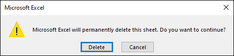
FIGURE 5-1: Omit the Application.DisplayAlerts = False line in the macro to ensure you get the opportunity to cancel the deletion.
To implement this macro, you can copy and paste it into a standard module. See the earlier section, “Installing Macros,” for more information.
Note that when you use ThisWorkbook in a macro rather than ActiveWorkbook, you can’t run the macro from the Personal Macro Workbook. This is because ThisWorkbook refers to the Personal Macro Workbook, not the workbook to which the macro should apply.
Hiding All but the Active Worksheet
You may not want to delete all but the active sheet as you did in the last macro. Instead, a more gentle option is to simply hide the sheets. Excel doesn't let you hide all sheets in a workbook; at least one has to be showing. However, you can hide all but the active sheet.
This macro loops the worksheets and matches each worksheet name to the active sheet’s name. Each time the macro loops, it hides any unmatched worksheet.
Sub HideAllButActiveSheet()

'Step 1: Declare your variables.
  Dim ws As Worksheet

'Step 2: Start looping through all worksheets.
  For Each ws In ThisWorkbook.Worksheets

'Step 3: Check each worksheet name.
    If ws.Name <> ThisWorkbook.ActiveSheet.Name Then

'Step 4: Hide the sheet.
      ws.Visible = xlSheetHidden
    End If

'Step 5: Loop to next worksheet.
  Next ws

End Sub
- Declares a Worksheet variable called ws. This creates a memory container for each worksheet the macro loops through.
The For Each keywords use the Worksheet control variable to loop through all the worksheets in the workbook. The loop runs once for every worksheet and on each pass the ws variable refers to a different worksheet.
There is a difference between ThisWorkbook and ActiveWorkbook. The ThisWorkBook object refers to the workbook that the code is contained in. The ActiveWorkBook object refers to the currently active workbook. They can return the same object, but if the workbook running the code is not the active workbook, they return different objects. In this case, you don’t want to risk deleting sheets in other workbooks, so be sure to use ThisWorkBook.- Compares the active sheet name to the sheet the loop is on.
- If the sheet names are different, the sheet is hidden.
The Next keyword tells Excel it's the end of the loop and to go back to the start if there are any worksheets yet to be evaluated. After all the sheets are evaluated, the macro ends.
 This example uses the built-in constant xlSheetHidden in the macro. This is the same as right-clicking a sheet and choosing Hide. Using this method means a user can right-click any tab and choose Unhide. But there is another, more clandestine, hidden state than the default. If you use xlSheetVeryHidden to hide your sheets, users won’t be able to see them at all — not even if they right-click any tab and choose Unhide. The only way to unhide a sheet hidden in this manner is to use VBA.
To implement this macro, you can copy and paste it into a standard module, as outlined in the first section in this chapter, “Installing Macros.”
Unhiding All Worksheets in a Workbook
You can unhide all hidden sheets by right-clicking a visible sheet and choosing Unhide to show the Unhide dialog box shown in Figure 5-2.
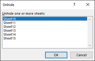
FIGURE 5-2: Without a macro, you’re stuck using Excel’s Unhide dialog box to unhide one worksheet at a time.
You can use the Shift and Ctrl keys to select multiple workbooks to unhide. If you want to save yourself some clicks, you can use this macro.
This macro loops the worksheets and makes sure each worksheet is visible.
Sub UnhideAllSheets()

'Step 1: Declare your variables.
  Dim ws As Worksheet

'Step 2: Start looping through all worksheets.
  For Each ws In ActiveWorkbook.Worksheets
'Step 3: Loop to next worksheet.
      ws.Visible = xlSheetVisible
  Next ws

End Sub
- Declares a Worksheet variable called ws. This creates a memory container for each worksheet the macro loops through.
- Uses For Each to tell Excel to enumerate through all worksheets in this workbook.
- Changes the Visible property to xlSheetVisible. Then loops to get the next worksheet.
The best place to store this macro is in your Personal Macro Workbook, as outlined in the first section of this chapter, “Installing Macros.” That way, the macro is always available to you.
Moving Worksheets Around
You’ve probably had to rearrange your workbook so that some sheets came before or after other sheets. If you find that you often have to do this, here is a macro that can help.
When you want to rearrange sheets, you use the Move method of either the Sheets object or the ActiveSheet object. When using the Move method, you need to specify where to move the sheet to. You can do this using the After argument, the Before argument, or you can omit both arguments. If you omit both, the worksheet is moved to a new workbook.
SSub MoveSheets()

'Move the active sheet to the end.
  ActiveSheet.Move After:=Worksheets(Worksheets.Count)

'Move the active sheet to the beginning.
  ActiveSheet.Move Before:=Worksheets(1)

'Move Sheet 1 before Sheet 12.
  Sheets("Sheet1").Move Before:=Sheets("Sheet12")

End Sub
This macro demonstrates how to move the active worksheet to three locations.
- Move the active sheet to the end: When you need to move a worksheet to the end of the workbook, Excel moves the sheet after the last sheet. There is no code in VBA that lets you point to “the last sheet.” But you can find the count of worksheets, and then use that number as an index for the Worksheets object. This means that you can enter something such as Worksheets(1) to point to the first sheet in a workbook. You can enter Worksheet(3) to point to the third sheet in the workbook. To point to the last sheet in the workbook, you can replace the index number with the Worksheets.Count property. Worksheets.Count gives you the total number of worksheets, which is the same number as the index for the last sheet. Thus Worksheet(Worksheets.Count) points to the last sheet.
- Move the active sheet to the beginning: Moving a sheet to the beginning of the workbook is simple. You use Worksheets(1) to point to the first sheet in the workbook, and then move the active sheet before that one.
- Move Sheet 1 before Sheet X: You can also move a sheet before or after another sheet simply by calling that other sheet by name. In the example demonstrated in the previous macro, Sheet1 is moved before Sheet12.
The best place to store this kind of macro is in your Personal Macro Workbook, as outlined in the first section of this chapter, “Installing Macros.” This way, the macro is always available to you.
Sorting Worksheets by Name
You may often need to sort worksheets alphabetically by name (see Figure 5-3). You would think Excel would have a native function to do this, but alas, it does not. If you don’t want to manually sort your spreadsheets anymore, you can use this macro to do it for you.
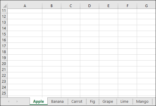
FIGURE 5-3: It’s often useful to have your worksheets sorted in alphabetical order.
This macro looks more complicated than it is. The activity in this macro is actually fairly simple. It iterates through the sheets in the workbook, comparing the current sheet to the previous one. If the name of the previous sheet is greater than the current sheet (alphabetically), the macro moves the current sheet before it. By the time all the iterations are done, you’ve got a sorted workbook!
Sub SortByName()

'Step 1: Declare your variables.
  Dim idxCurr As Long
  Dim idxPrev As Long

'Step 2: Set the starting counts and start looping.
  For idxCurr = 2 To Sheets.Count
    For idxPrev = 1 To idxCurr - 1

'Step 3: Check current sheet against previous sheet.
      If UCase(Sheets(idxPrev).Name) > _
        UCase(Sheets(idxCurr).Name) Then

'Step 4: If move current sheet before previous.
        Sheets(idxCurr).Move _
          Before:=Sheets(idxPrev)
      End If

'Step 5: Loop back around to iterate again
    Next idxPrev
  Next idxCurr

End Sub
Note this technique is doing a text-based sorting. So you may not get the results you were expecting when working with number-based sheet names. For example, Sheet10 comes before Sheet2 because textually, 1 comes before 2. Excel does not do the numbers-based sorting that says 2 comes before 10.
- Declares two Long variables. The idxCurr variable holds the index number for the current sheet iteration, and the idxPrev variable holds the index number for the previous sheet iteration.
- Creates an outer loop using idxCurr and an inner loop using idxPrev. The outer loop starts at 2 so you don't compare the first sheet to itself and the inner loop stops one before the end so you don't compare the last sheet to itself.
Checks to see whether the name of the previous sheet is greater than that of the current sheet.
Use the UCase function to get both names in uppercase. This prevents sorting errors due to differing cases.- If the previous sheet name is greater than the current sheet name, the Move method moves the current sheet before the previous sheet.
- Goes back to the start of the loop. Every iteration of the loop increments both variables up one number until the last worksheet is touched. After all iterations have been spent, the macro ends.
The best place to store this macro is in your Personal Macro Workbook, as outlined in the first section of this chapter, “Installing Macros.” This way, the macro is always available to you.
Grouping Worksheets by Color
This macro is useful if you assign colors to your worksheet tabs. You can right-click any tab and select the Tab Color option (shown in Figure 5-4) to choose a color for your tab.

FIGURE 5-4: You can right-click any worksheet to choose a tab color for the sheet.
This allows for visual confirmation that the data in a certain tab is somehow related to another tab because both have the same color. When you have many colored sheets, it’s often useful to group tabs of similar color together for ease of navigation.
This macro groups worksheets based on their tab colors. You may think it's impossible to sort or group by color, but Excel offers a way. Excel assigns an index number to every color. A light yellow color may have an index number of 36, whereas a maroon color has the index number 42.
This macro iterates through the sheets in the workbook, comparing the tab color index of the current sheet to that of the previous one. If the previous sheet has the same color index number as the current sheet, the macro moves the current sheet before it. By the time all the iterations are done, all the sheets are grouped together based on their tab colors.
Sub GroupByColor()

'Step 1: Declare your variables.
  Dim idxCurr As Long
  Dim idxPrev As Long

'Step 2: Set the starting counts and start looping.
  For idxCurr = 2 To Sheets.Count
    For idxPrev = 1 To idxCurr - 1

'Step 3: Check current sheet against previous sheet.
      If Sheets(idxPrev).Tab.ColorIndex = _
        Sheets(idxCurr).Tab.ColorIndex Then

'Step 4: Move current sheet before previous.
        Sheets(idxPrev).Move _
          Before:=Sheets(idxCurr)
      End If

'Step 5: Loop back around to iterate again.
    Next idxPrev
  Next idxCurr

End Sub
- Declares two Long variables. The idxCurr variable holds the index number for the current sheet iteration, and the idxPrev variable holds the index number for the previous sheet iteration.
- Creates an outer loop using idxCurr and an inner loop using idxPrev. The outer loop starts at 2 so you don't compare the first sheet to itself and the inner loop stops one before the end so you don't compare the last sheet to itself.
- Checks to see whether the color index of the previous sheet is the same as that of the current sheet using the Tab.ColorIndex property.
- If the color index of the previous sheet is equal to the color index of the current sheet, the Move method moves the current sheet before the previous sheet.
- Goes back to the start of the loop. Every iteration of the loop increments both variables up one number until the last worksheet is touched. After all iterations have been spent, the macro ends.
The best place to store this macro is in your Personal Macro Workbook, as outlined in the first section of this chapter, “Installing Macros.” This way, the macro is always available to you.
Copying a Worksheet to a New Workbook
In Excel, you can manually copy an entire sheet to a new workbook by right-clicking the target sheet and selecting the Move or Copy option. Unfortunately, if you try to record a macro while you do this, the macro recorder fails to accurately write the code to reflect the task. So if you need to programmatically copy an entire sheet to a brand new workbook, this macro delivers.
In this macro, the active sheet is first being copied. Then you use the Before parameter to send the copy to a new workbook that is created on the fly. The copied sheet is positioned as the first sheet in the new workbook.
The use of the ThisWorkbook object is important here. This ensures that the active sheet being copied is from the workbook that the code is in, not the newly created workbook.
Sub CopySheetToNewWb()

'Copy sheet, and send to new workbook.
  ThisWorkbook.ActiveSheet.Copy _
    Before:=Workbooks.Add.Worksheets(1)

End Sub
To implement this macro, you can copy and paste it into a standard module. See the first section in this chapter, “Installing Macros,” for more information.
Creating a New Workbook for Each Worksheet
Many Excel analysts need to parse their workbooks into separate books per worksheet tab. In other words, they need to create a new workbook for each of the worksheets in their existing workbook. You can imagine what an ordeal this would be if you were to do it manually. The following macro helps automate that task.
In this macro, you are looping the worksheets, copying each sheet, and then sending the copy to a new workbook that is created on the fly. The thing to note here is that the newly created workbooks are being saved in the same directory as your original workbook, with the same filename as the copied sheet (wb.SaveAs ThisWorkbook.Path & "" & ws.Name).
Sub NewWbForEachSheet()

'Step 1: Declare all the variables.
  Dim ws As Worksheet
  Dim wb As Workbook

'Step 2: Start the looping through sheets.
  For Each ws In ThisWorkbook.Worksheets

'Step 3: Create new workbook and save it.
    Set wb = Workbooks.Add
    wb.SaveAs ThisWorkbook.Path & "" & ws.Name

'Step 4: Copy the target sheet to the new workbook.
    ws.Copy Before:=wb.Worksheets(1)
    wb.Close SaveChanges:=True

'Step 5: Loop back around to the next worksheet.
  Next ws

End Sub
Not all valid worksheet names translate to valid filenames.
Windows has specific rules that prevent you from naming files with certain characters. You cannot use these characters when naming a file: back slash (), forward slash (/), colon (:), asterisk (*), question mark (?), pipe (|), double quote (“), greater than (>), and less than (<).
The twist is that you can use a few of these restricted characters in your sheet names; specifically, double quote (“), pipe (|), greater than (>), and less than (<).
So as you’re running this macro, naming the newly created files to match the sheet name may cause an error. For example, the macro throws an error when creating a new file from a sheet called “May| Revenue” (because of the pipe character).
Long story short, avoid naming your worksheets with the restricted characters just mentioned.
- Declares two object variables. The ws variable creates a memory container for each worksheet the macro loops through. The wb variable creates the container for the new workbooks you create.
- Loops through the sheets. The use of the ThisWorkbook object ensures that the active sheet being copied is from the workbook the code is in, not the newly created workbook.
- Adds a new workbook and save it. You save this new book in the same path as the original workbook (ThisWorkbook). The filename is set to be the same name as the currently active sheet.
- Copies the currently active sheet, using the Before parameter to send it to the new book as the first sheet. Then saves and closes the newly created workbook.
- Loops back to get the next sheet. After all of the sheets are evaluated, the macro ends.
To implement this macro, you can copy and paste it into a standard module. See the earlier section, “Installing Macros,” to find out how.
Printing Specified Worksheets
If you want to print specific sheets manually in Excel, you need to hold down the Ctrl key on the keyboard, select the sheets you want to print, and then click Print. If you do this often enough, you may consider using this very simple macro.
This one is easy. All you have to do is pass the sheets you want printed in an array as seen here in this macro, and then use the PrintOut method to trigger the print job. All the sheets you have entered are printed in one go.
Sub PrintSheets()

'Print certain sheets.
  ActiveWorkbook.Sheets( _
    Array("Sheet1", "Sheet3", "Sheet5")).PrintOut Copies:=1

End Sub
Want to print all worksheets in a workbook? This one is even easier.
Sub PrintAllSheets()

'Print all sheets.
  ActiveWorkbook.Worksheets.PrintOut Copies:=1

End Sub
The best place to store this macro is in your Personal Macro Workbook, as outlined in the first section of this chapter, “Installing Macros.” This way, the macro is always available to you.
Protecting All Worksheets
Before you distribute your workbook, you may want to apply sheet protection to all the sheets. However, as shown in Figure 5-5, Excel disables the Protect Sheet command if you try to protect multiple sheets at one time. You’re forced to protect one sheet at a time. You can use this macro to save you from protecting each sheet manually.
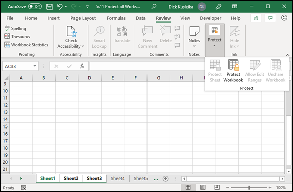
FIGURE 5-5: The Protect Sheet command is disabled if you try to protect more than one sheet at a time.
In this macro, you’re looping the worksheets and simply applying protection with a password. The Password argument defines the password needed to remove the protection. The Password argument is completely optional. If you omit it altogether, the sheet is still protected; you just won’t need to enter a password to unprotect it. Also, be aware that Excel passwords are case-sensitive, so you want pay attention to the exact capitalization you are using.
Sub ProtectAllSheets()

'Step 1: Declare your variables.
  Dim ws As Worksheet

'Step 2: Start looping through all worksheets.
  For Each ws In ActiveWorkbook.Worksheets

'Step 3: Protect and loop to next worksheet.
    ws.Protect Password:="RED"
  Next ws

End Sub
- Declares a Worksheet variable called ws. This creates a memory container for each worksheet you loop through.
- Starts the looping, telling Excel you want to enumerate through all worksheets in this workbook.
- Applies protection with the given password, and then loops back to get the next worksheet.
The best place to store this macro is in your Personal Macro Workbook, as outlined in the first section of this chapter, “Installing Macros.” This way, the macro is always available to you.
Unprotecting All Worksheets
You may find yourself constantly having to unprotect multiple worksheets manually. However, as shown in Figure 5-6, Excel disables the Unprotect Sheet command if you try to unprotect multiple sheets at one time. You’re forced to unprotect one sheet at a time. You can use this macro to save you from unprotecting each sheet manually.
This macro loops the worksheets and uses the Password argument to unprotect each sheet.
Sub UnprotectAllSheets()

'Step 1: Declare your variables.
  Dim ws As Worksheet

'Step 2: Start looping through all worksheets.
  For Each ws In ActiveWorkbook.Worksheets

'Step 3: Loop to next worksheet.
    ws.Unprotect Password:="RED"
  Next ws

End Sub
- Declares an Worksheet variable called ws. This creates a memory container for each worksheet you loop through.
- Starts the looping, telling Excel to enumerate through all worksheets in this workbook.
- Unprotects the active sheet, providing the password as needed, and then loops back to get the worksheet.
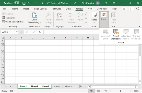
FIGURE 5-6: The Unprotect Sheet command is disabled if you try to unprotect more than one sheet at a time.
Obviously, the assumption is that all the worksheets that need to be unprotected have the same password. If this is not the case, you need to explicitly unprotect each sheet with its corresponding password.
Sub UnprotectAllSheets2()

  Sheets("Sheet1").Unprotect Password:="RED"
  Sheets("Sheet2").Unprotect Password:="BLUE"
  Sheets("Sheet3").Unprotect Password:="YELLOW"
  Sheets("Sheet4").Unprotect Password:="GREEN"

End Sub
The best place to store this kind of a macro is in your Personal Macro Workbook, as outlined in the first section of this chapter, “Installing Macros.” This way, the macro is always available to you.
Creating a Table of Contents for Your Worksheets
Outside of sorting worksheets, creating a table of contents for the worksheets in a workbook is the most commonly requested Excel macro. The reason is probably not lost on you if you often work with files that have more worksheet tabs than can easily be seen or navigated. A table of contents such as the one shown in Figure 5-7 definitely helps.
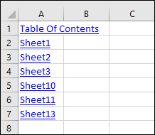
FIGURE 5-7: A table of contents can help you more easily navigate your workbook.
The following macro not only creates a list of worksheet names in the workbook, but it also adds hyperlinks so that you can easily jump to a sheet with a simple click.
It’s easy to get intimidated when looking at this macro. A lot is going on here. However, if you step back and consider the few simple actions it does, it becomes a little less scary:
- It removes any previous Table of Contents sheet.
- It creates a new Table of Contents sheet.
- It grabs the name of each worksheet and pastes it on the Table of Contents.
- It adds a hyperlink to each entry in the Table of Contents.
That doesn’t sound so bad. Now look at the code:
Sub CreateTOC()

'Step 1: Declare variables.
  Dim i As Long

'Step 2: Delete previous TOC if exists.
  On Error Resume Next
    Application.DisplayAlerts = False
    Sheets("Table Of Contents").Delete
    Application.DisplayAlerts = True
  On Error GoTo 0

'Step 3: Add a new TOC sheet as the first sheet.
  ThisWorkbook.Sheets.Add _
    Before:=ThisWorkbook.Worksheets(1)
  ActiveSheet.Name = "Table Of Contents"

'Step 4: Start the i counter.
  For i = 1 To Sheets.Count

'Step 5: Select next available row.
    ActiveSheet.Cells(i, 1).Select

'Step 6: Add sheet name and hyperlink.
    ActiveSheet.Hyperlinks.Add _
      Anchor:=ActiveSheet.Cells(i, 1), _
      Address:="", _
      SubAddress:="'" & Sheets(i).Name & "'!A1", _
      TextToDisplay:=Sheets(i).Name

'Step 7: Loop back increment i.
  Next i

End Sub
Declares a Long integer variable called i to serve as the counter as the macro iterates through the sheets.
Note that this macro is not looping through the sheets the way previous macros in this chapter did. In previous macros, you looped through the worksheets collection and selected each worksheet there. This macro uses a counter (your i variable). The main reason is because you not only have to keep track of the sheets, but you also have to manage to enter each sheet name on a new row into a table of contents. The idea is that as the counter progresses through the sheets, it also serves to move the cursor down in the Table of Contents so each new entry goes on a new row.- Attempts to delete any previous sheet called Table of Contents. Because there may not be any Table of Contents sheet to delete, you have to start with the On Error Resume Next error statement. This tells Excel to continue the macro if an error is encountered here. You then set DisplayAlerts to False so you don’t have to confirm the deletion. Delete the sheet and reset DisplayAlerts and the error handler to trap all errors again by entering On Error GoTo 0.
- Adds a new sheet to the workbook using the Before argument to position the new sheet as first sheet. Name the sheet Table of Contents. Remember that when you add a new worksheet, it automatically becomes the active sheet. Because this new sheet has the focus throughout the macro, any references to ActiveSheet in this code refer to the Table of Contents sheet.
- Starts the i counter at 1 and ends it at the count of all sheets in the workbook. Again, instead of looping through the Worksheets collection like in previous macros, the i counter stores an index number that is passed to the Sheets object. When the maximum number is reached, the macro ends.
Selects the corresponding row in the Table of Contents sheet. That is to say, if the i counter is on 1, it selects the first row in the Table of Contents sheet. If the i counter is at 2, it selects the second row, and so on.
You are able to do this using the Cells property. The Cells property provides an extremely handy way of selecting ranges through code. It requires only relative row and column positions as parameters. So Cells(1,1) translates to row 1, column 1 (or cell A1). Cells(5, 3) translates to row 5, column 3 (or cell C5).
The numeric parameters in the Cells item are particularly handy when you want to loop through a series of rows or columns using an incrementing index number.- Adds a hyperlink using the Hyperlinks.Add method to add the sheet name and hyperlinks to the selected cell. The Anchor parameter determines which cell the hyperlink is in. The Address is blank because all the links are within the workbook that contains the hyperlink. To link outside of the workbook, set the Address property to the other file. The SubAddress is the sheet name and cell address within the file. The TextToDisplay argument is what shows in the hyperlink cell.
- Loops back to increment the i counter to the next count. When the i counter reaches a number that equals the count of worksheets in the workbook, the macro ends.
To implement this macro, you can copy and paste it into a standard module. See the section at the beginning of this chapter, “Installing Macros,” for details.
Zooming In and Out of a Worksheet with Double-Click
Some spreadsheets are huge. Sometimes, you’re forced to shrink the font size down so that you can see a decent portion of the spreadsheet onscreen. If you find that you’re constantly zooming in and out of a spreadsheet, alternating between scanning large sections of data and reading specific cells, here is a handy macro that auto-zooms on double-click.
With this macro in place, you can double-click a cell in the spreadsheet to zoom in 200 percent. Double-click again and Excel zooms out to 100 percent. Obviously, you can change the values and complexity in the code to fit your needs.
Private Sub Worksheet_BeforeDoubleClick(ByVal Target As Range, _
  Cancel As Boolean)

'Check current zoom state
'Zoom to 100% if not at 100
'Zoom 200% if currently at 100
  If ActiveWindow.Zoom <> 100 Then
    ActiveWindow.Zoom = 100
  Else
    ActiveWindow.Zoom = 200
  End If

  Cancel = True
End Sub
The default behavior of double-clicking a cell is that it goes into edit mode. This macro sets the Cancel argument to True to prevent that behavior.
To implement this macro, you need to copy and paste it into the Worksheet_BeforeDoubleClick event Code pane, as shown in Figure 5-8. See the first section at the beginning of this chapter, “Installing Macros,” for more information. Placing the macro there allows it to run each time you double-click the sheet.
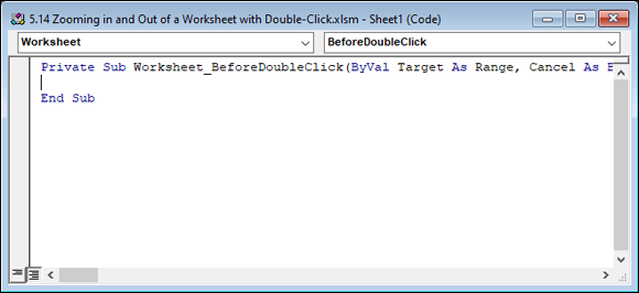
FIGURE 5-8: Type or paste your code into the Worksheet_BeforeDoubleClick event code window.
Highlighting the Active Row and Column
When looking at a table of numbers, it would be nice if Excel automatically highlighted the row and column you’re on (as shown in Figure 5-9). This effect gives your eyes a lead line up and down the column as well as left and right across the row.

FIGURE 5-9: A highlighted row and column makes it easy to track data horizontally and vertically.
The following macro enables the effect shown in Figure 5-9 with just a simple double-click. When the macro is in place, Excel highlights the row and column for the active cell, greatly improving your ability to view and edit a large grid.
Take a look at how this macro works:
Private Sub Worksheet_BeforeDoubleClick(ByVal Target As Range, Cancel As Boolean)

  Application.Union(Target.EntireColumn, _
    Target.EntireRow).Select

End Sub
The Union method takes multiple ranges of cells and makes them a single range of cells. In this example, it takes the whole column and the whole row and creates one range containing both. Then it's a simple call to the Select method to highlight the range.
To implement this macro, you need to copy and paste it into the Worksheet_BeforeDoubleClick event Code pane. See the first section in this chapter, “Installing Macros,” for more information. Placing the macro there allows it to run each time you double-click the sheet.