
Chapter 13
Using External Data for Your Dashboards and Reports
In This Chapter
![]() Importing from Microsoft Access
Importing from Microsoft Access
![]() Importing from SQL Server
Importing from SQL Server
![]() Leveraging Power Query to get external data
Leveraging Power Query to get external data
Wouldn’t it be wonderful if all the data you come across could be neatly packed into one easy-to-use Excel table? The reality is that sometimes the data you need comes from external data sources. External data is exactly what it sounds like: data that isn’t located in the Excel workbook in which you’re operating. Some examples of external data sources are text files, Access tables, SQL Server tables, and even other Excel workbooks.
This chapter explores some efficient ways to get external data into your Excel data models. Before jumping in, however, this humble author wants to throw out one disclaimer: There are numerous ways to get data into Excel. In fact, between the functionality found in the user interface and the VBA/code techniques, Excel has too many techniques to focus on in one chapter. Instead, then, in this chapter I focus on a handful of techniques that can be implemented in most situations and don’t come with a lot of pitfalls and gotchas.
Importing Data from Microsoft Access
Microsoft Access is used in many organizations to manage a series of tables that interact with each other, such as a Customers table, an Orders table, and an Invoices table. Managing data in Access provides the benefit of a relational database in which you can ensure data integrity, prevent redundancy, and easily generate datasets via queries.
Excel offers several methods for getting your Access data into your Excel data model.
The drag-and-drop method
For simplicity, you just can’t beat the drag-and-drop method. You can simultaneously open an empty Excel workbook and an Access database from which you want to import a table or query. When both are open, resize each application’s window so that they’re both fully visible on your screen.
Hover the mouse pointer over the Access table or query you want to copy into Excel. Now click the table and drag it to the blank worksheet in Excel, as illustrated in Figure 13-1.

Figure 13-1: Copy an Access table using the drag-and-drop method.
The drag-and-drop method comes in handy when you’re doing a quick one-time analysis in which you need a specific set of data in Excel. However, the method isn’t so useful under the following conditions:
- You expect this step to occur routinely, as part of a repeated analysis or report.
- You expect the users of your Excel presentation to get or update the data via this method.
- It’s not possible or convenient for you to simply open up Access every time you need the information.
In these scenarios, it’s much better to use another technique.
The Microsoft Access Export wizard
Access has an Export wizard, and it’s relatively simple to use. Just follow these steps:
- With your Access database open, click your target table or query to select it.
-
On the External Data tab on the Ribbon, select the Excel icon under the Export group.
The wizard that you see in Figure 13-2 opens.
As you can see in Figure 13-2, you can specify certain options in the Excel Export wizard. You can specify the file location, the file type, and some format preservation options.
- In the Excel Export Wizard, select Export Data with Formatting and Layout and then select Open the Destination File After the Export Operation is Complete.
-
Click OK.
Excel opens to show you the exported data.

Figure 13-2: Export data to Excel using the Excel Export Wizard.
 In Access, the last page in the Export wizard, shown in Figure 13-3, asks whether you want to save your export steps. Saving your export steps can be useful if you expect to frequently send that particular query or table to Excel. The benefit to this method is that unlike dragging and dropping, the ability to save export steps allows you to automate your exports by using Access macros.

Figure 13-3: Use the Save Export Steps option if you export your data frequently.
 You may export your Access table or query to an existing Excel file instead of creating a new file. But note that the name of the exported object will be the name of the table or query in Access. Be careful if you have an Excel object with that same name in your workbook, because it may be overwritten. For example, exporting an Access table named PriceMaster to an Excel worksheet that already has a worksheet named PriceMaster causes the original Excel PriceMaster worksheet to be overwritten. Also, make sure the workbook to which you’re exporting is closed. If you try to export to an open workbook, you’ll likely receive an error in Access.
The Get External Data icon
The option to pull data from Access has been available in Excel for many versions; it was just buried several layers deep in somewhat cryptic menu titles. This made getting Access data into Excel seem like a mysterious and tenuous proposition for many Excel analysts. With the introduction of the Ribbon in Excel 2007, Microsoft put the Get External Data group of commands right on the Ribbon under the Data tab, making it easier to import data from Access and other external data sources.
Excel allows you to establish an updatable data connection between Excel and Access. To see the power of this technique, walk through these steps:
- Open a new Excel workbook and click the Data tab on the Ribbon.
-
In the Get External Data group, select the From Access icon.
The Select Data Source dialog box opens. If the database from which you want to import data is local, browse to the file’s location and select it. If your target Access database resides on a network drive at another location, you need the proper authorization to select it.
-
Navigate to the sample database and click Open, as shown in Figure 13-4.
In some environments, a series of Data Link Properties dialog boxes opens, asking for credentials (that is, username and password). Most Access databases don’t require logon credentials, but if your database does require a username and password, type them in the Data Link Properties dialog box.
-
Click OK.
The Select Table dialog box shown in Figure 13-5 opens. This dialog box lists all available tables and queries in the selected database.
 The Select Table dialog box contains a column called Type. There are two types of Access objects you can work with: views and tables. VIEW indicates that the dataset listed is an Access query, and TABLE indicates that the dataset is an Access table. In this example, Sales_By_Employee is actually an Access query. This means that you import the results of the query. This is true interaction at work; Access does all the back-end data management and aggregation, and Excel handles the analysis and presentation!
 -
Using the Select Table dialog box, select your target table or query and then click OK.
The Import Data dialog box shown in Figure 13-6 opens. There, you define where and how to import the table. You have the option to import the data into a Table, a PivotTable Report, a PivotChart, or a Power View Report. You also have the option to create only the connection, making the connection available for later use.
Note that if you choose PivotChart or PivotTable Report, the data is saved to a pivot cache without writing the actual data to the worksheet. Thus, the pivot table can function as normal without your having to import potentially hundreds of thousands of data rows twice (once for the pivot cache and once for the spreadsheet).
- Select Table as the output view and define cell A1 as the output location. Refer to Figure 13-6.
-
Click OK.
The reward for all your work is a table similar to the one shown in Figure 13-7, which contains the imported data from your Access database.

Figure 13-4: Choose your source database.

Figure 13-5: Select the Access object you want to import.

Figure 13-6: Choosing how and where to view your Access data.

Figure 13-7: Your imported Access data.
The incredibly powerful thing about importing data this way is that it’s refreshable. That’s right: If you import data from Access using this technique, Excel creates a table that you can update by right-clicking it and selecting Refresh from the pop-up menu, as shown in Figure 13-8. When you update your imported data, Excel reconnects to your Access database and imports the data again. As long as a connection to your database is available, you can refresh with a mere click of the mouse.

Figure 13-8: As long as a connection to your database is available, you can update your table with the latest data.
Again, a major advantage to using the Get External Data group is that you can establish a refreshable data connection between Excel and Access. In most cases, you can set up the connection one time and then just update the data connection when needed. You can even record an Excel macro to update the data on some trigger or event, which is ideal for automating the transfer of data from Access.
Importing Data from SQL Server
In the spirit of collaboration, Excel vastly improves your ability to connect to transactional databases such as SQL Server. With the connection functionality found in Excel, creating a connected table or pivot table from SQL Server data is as easy as ever.
Start on the Data tab and follow these steps:
-
Click the From Other Sources icon to see the drop-down menu shown in Figure 13-9; then select From SQL Server.
Selecting this option activates the Data Connection Wizard, as shown in Figure 13-10. There, you configure the connection settings so that Excel can establish a link to the server.
-
Provide Excel with some authentication information.
Enter the name of your server as well as your username and password; see Figure 13-10. If you’re typically authenticated via Windows authentication, however, simply select the Use Windows Authentication option.
-
Select the database with which you’re working from a drop-down menu containing all available databases on the specified server.
As you can see in Figure 13-11, a database called AdventureWorks2012 is selected in the drop-down box. All the tables and views in this database are shown in the list of objects below the drop-down menu.
- Choose the table or view you want to analyze and then click Next.
-
On the screen that appears in the wizard, enter descriptive information about the connection you’ve just created. (See Figure 13-12 for an example.)
This information is optional. If you bypass this screen without editing anything, your connection will work fine.
The fields that you use most often in this particular screen are
- File Name: In the File Name input box, you can change the filename of the ODC (Office Data Connection) file generated to store the configuration information for the link you just created.
- Save Password in File: Under the File Name input box, you have the option of saving the password for your external data in the file itself (via the Save Password in File check box). Selecting this check box actually enters your password in the file. This password is not encrypted, so anyone interested enough could potentially get the password for your data source by simply viewing the file with a text editor.
- Description: In the Description field, you can enter a plain description of what this particular data connection does.
- Friendly Name: The Friendly Name field allows you to specify a name of your own choosing for the external source. You typically enter a name that is descriptive and easy to read.
-
When you are satisfied with your descriptive edits, click Finish to finalize your connection settings.
You immediately see the Import Data dialog box, where you can choose how to import data. As you can see in Figure 13-13, this data will be shown in a pivot table.
When the connection is finalized, you can start building your pivot table.

Figure 13-9: Select the From SQL Server option from the drop-down menu.

Figure 13-10: Enter your authentication information and click Next.

Figure 13-11: Specify your database and then choose the table or view you want to analyze.

Figure 13-12: Enter descriptive information for your connection.

Figure 13-13: Choosing how and where to view your SQL Server data.
Leveraging Power Query to Extract and Transform Data
Every day, millions of Excel users manually pull data from some source location, manipulate that data, and integrate it into their pivot table reporting.
This process of extracting, manipulating, and integrating data is called ETL. ETL refers to the three separate functions typically required in order to integrate disparate data sources: extract, transform, and load.
- The extraction function involves reading data from a specified source and extracting a desired subset of data.
- The transformation function involves cleaning, shaping, and aggregating data to convert it to the desired structure.
- The loading function involves actually importing or using the resulting data.
In an attempt to empower Excel analysts to develop robust and reusable ETL processes, Microsoft created Power Query. Power Query enhances the ETL experience by offering an intuitive mechanism to extract data from a wide variety of sources, perform complex transformations on that data, and then load the data into a workbook or the internal Data Model.
In this section, you see how Power Query works and how you can use it to help save time and automate the steps for importing data into your reporting models.
Reviewing Power Query basics
Although Power Query is relatively intuitive, it’s worth taking the time to walk through a basic scenario to understand its high-level features. To start this basic look at Power Query, pretend that your job entails creating reports that show trending for Microsoft stock prices. As a part of your job, you frequently need to pull stock data from the web.
Follow these steps to start a query to pull the needed stock data from Yahoo! Finance:
-
Select the New Query command on the Data tab and then select From Other Sources ⇒ From Web, as shown in Figure 13-14.
Excel has another From Web command button on the Data tab under the Get External Data group. This unfortunate duplicate command is actually the legacy web-scraping capability found in all Excel versions going back to Excel 2000. The Power Query version of the From Web command (found under New Query ⇒ From Other Sources ⇒ From Web) goes beyond simple web scraping. Power Query is able to pull data from advanced web pages and is able to manipulate the data. Make sure you are using the correct feature when pulling data from the web. -
In the dialog box that appears (see Figure 13-15), enter the URL for the data you need (in this case,
http://finance.yahoo.com/q/hp?s=MSFT).After a bit of gyrating, the Navigator pane shown in Figure 13-16 appears.
-
Using the Navigator pane, select the data source you want extracted.
You can click each table to see a preview of the data. In this case, Table 4 holds the historical stock data you need, so click Table 4 and then click the Edit button.
When you click the Edit button, Power Query activates a new Query Editor window, which contains its own Ribbon and a preview pane that shows a preview of the data. (See Figure 13-17.) Here, you can apply certain actions to shape, clean, and transform the data before importing.
The idea is to work with each column shown in the Query Editor, applying the necessary actions that will give you the data and structure you need. You’ll dive deeper into column actions later in this chapter. For now, you need to continue toward the goal of getting the last 30 days of stock prices for Microsoft Corporation.
You may have noticed that the Navigator pane shown in Figure 13-16 offers a Load button (next to the Edit button). The Load button allows you to skip any editing and import your targeted data as is. If you are sure you will not need to transform or shape your data in any way, you can opt to click the Load button to import the data directly into the Data Model or a spreadsheet in your workbook. - Right-click the Date field to see the available column actions, as shown in Figure 13-18, and then choose Change Type ⇒ Date to ensure that the Date field is formatted as a proper date.
-
Remove all columns you do not need by right-clicking each one and selecting Remove from the menu that appears.
Besides the Date field, the only columns you need are the High, Low, and Close fields. Alternatively, you can hold down the Ctrl key on the keyboard, select the columns you want to keep, right-click any selected column, and then choose Remove Other Columns from the menu that appears. (See Figure 13-19.)
-
Ensure that the High, Low, and Close fields are formatted as proper numbers. To do this, hold down the Ctrl key on the keyboard, select the three columns, right-click, and then choose Change Type ⇒ Decimal Number from the menu that appears.
After you do this, you may notice that some of the rows show the word Error. These are rows that contained text values that could not be converted.
- Remove the Error rows by selecting Remove Errors from the Table Actions list (next to the Date field), as shown in Figure 13-20.
-
After all errors are removed, add a Week Of field that displays the week each date in the table belongs to. To do this, right-click the Date field and select the Duplicate Column option.
Doing so adds a new column to the preview.
- Right-click the newly added column, select the Rename option from the menu that appears, and then rename the column Week Of.
-
Select the Transform tab on the Power Query ribbon and then choose Date ⇒ Week ⇒ Start of the Week, as shown in Figure 13-21.
Excel transforms the date to display the start of the week for a given date.
-
When you’ve finished configuring your Power Query feed, save and output the results. To do this, click the Close & Load drop-down found on the Home tab of the Power Query ribbon to reveal the two options shown in Figure 13-22.
The Close & Load option saves your query and outputs the results as an Excel table to a new worksheet in your workbook.
The Close & Load To gives you the option of saving your output results to the internal data model.

Figure 13-14: Starting a Power Query web query.

Figure 13-15: Enter the target URL containing the data you need.
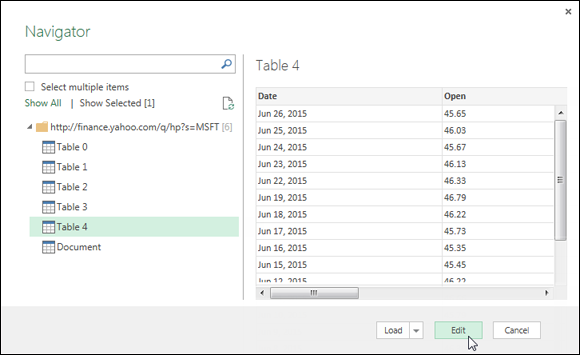
Figure 13-16: Select the correct data source and then click the Edit button.

Figure 13-17: The Query Editor window allows you to shape, clean, and transform data.

Figure 13-18: Right-click the Date column and choose to change the data type to a date format.

Figure 13-19: Select the columns you do not want to keep and then select Remove Other Columns to get rid of them.

Figure 13-20: You can click the Table Actions icon to select actions (such as Remove Errors) that you want applied to the entire data table.

Figure 13-21: The Power Query ribbon can be used to apply transformation actions such as displaying the start of the week for a given date.

Figure 13-22: Select the Close & Load option to output your results as a table on a new worksheet.
At this point, you should have a table similar to the one shown in Figure 13-23, which can be used to produce the pivot table you need.

Figure 13-23: Your final query extracted from the Internet, transformed, and loaded into an Excel table.
Take a moment to appreciate what Power Query allowed you to do just now. With a few clicks, you searched the Internet, found some base data, shaped the data to keep only the columns you needed, and even manipulated that data to add an extra Week Of dimension to the base data. This is what Power Query is about: enabling you to easily extract, filter, and reshape data without the need for any programmatic coding skills.
Understanding query steps
Power Query uses its own formula language (known as the “M” language) to codify your queries. As with macro recording, each action you take when working with Power Query results in a line of code being written into a query step. Query steps are embedded M code that allow your actions to be repeated every time you refresh your Power Query data.
You can see the query steps for your queries by activating the Query Settings pane. Simply click the Query Settings command on the View tab of the Query Editor ribbon. You can also place a check in the Formula Bar option to enhance your analysis of each step with a formula bar that displays the syntax for the given step.
The Query Settings pane appears to the right of the Preview pane, as shown in Figure 13-24. The formula bar is located directly above the Preview pane.

Figure 13-24: Query steps can be viewed and managed in the Applied Steps section of the Query Settings pane.
Each query step represents an action you took to get to a data table. You can click any step to see the underlying M code in the Power Query formula bar. For example, clicking the step called Removed Errors reveals the code for that step on the formula bar.
When you click a query step, the data shown in the preview pane is a preview of what the data looked like up to and including the step you clicked. For example, in Figure 13-24, clicking the step before the Removed Other Columns step lets you see what the data looked like before you removed the nonessential columns.
You can right-click on any step to see a menu of options for managing your query steps. Figure 13-25 illustrates the following options:
- Edit Settings: Edits the arguments or parameters that define the selected step.
- Rename: Gives the selected step a meaningful name.
- Delete: Removes the selected step. Be aware that removing a step can cause errors if subsequent steps depend on the deleted step.
- Delete Until End: Removes the selected step and all following steps.
- Move Up: Moves the selected step up in the order of steps.
- Move Down: Moves the selected step down in the order of steps.

Figure 13-25: Right-click any query step to edit, rename, delete, or move the step.
Refreshing Power Query data
It’s important to note that Power Query data is not in any way connected to the source data used to extract it. A Power Query data table is merely a snapshot. In other words, as the source data changes, Power Query doesn’t automatically keep up with the changes; you need to intentionally refresh your query.
If you chose to load your Power Query results to an Excel table in the existing workbook, you can manually refresh by right-clicking the table and selecting the Refresh option from the menu that appears.
If you chose to load your Power Query data to the internal Data Model, you need to open the Power Pivot window, select your Power Query data, and then click the Refresh command on the Home tab of the Power Query window.
To get a bit more automated with the refreshing of your queries, you can configure your data sources to automatically refresh your Power Query data. To do so, follow these steps:
-
Go to the Data tab on the Excel ribbon and select the Connections command.
The Workbook Connections dialog box appears.
- Select the Power Query data connection you want to refresh and then click the Properties button.
- With the Properties dialog box open, select the Usage tab.
-
Set the following options to refresh the chosen data connection. (See Figure 13-26):
- Refresh Every X Minutes: Placing a check mark next to this option tells Excel to automatically refresh the chosen data every specified number of minutes. Note that Excel refreshes all tables associated with that connection.
- Refresh Data When Opening the File: Placing a check mark next to this option tells Excel to automatically refresh the chosen data connection upon opening the workbook. Excel refreshes all tables associated with that connection as soon as the workbook is opened.
These refresh options are useful when you want to ensure that your customers are working with the latest data. Of course, setting these options doesn’t preclude the ability to manually refresh the data using the Refresh command on the Home tab.

Figure 13-26: You can tell Excel to automatically refresh your query when opening the workbook or at a specified interval.
Managing existing queries
As you add various queries to a workbook, you need a way to manage them. Excel accommodates this need by offering the Workbook Queries pane, which enables you to edit, duplicate, refresh, and generally manage all existing queries in the workbook. Activate the Workbook Queries pane by selecting the Show Queries command on the Data tab of the Excel ribbon.
The idea is to find the query you want to work with and then right-click the query to take any one of the actions shown in Figure 13-27.

Figure 13-27: Right-click any query in the Workbook Queries pane to see the available management options.
- Edit: Opens the Query Editor, where you can modify the query steps
- Delete: Deletes the selected query
- Refresh: Refreshes the data in the selected query
- Load To: Activates the Load To dialog box, where you can redefine where the selected query’s results are used
- Duplicate: Creates a copy of the query
- Reference: Creates a new query that references the output of the original query
- Merge: Merges the selected query with another query in the workbook by matching specified columns
- Append: Appends the results of another query in the workbook to the selected query
- Send to Data Catalog: Publishes and shares the selected query via a Power BI server that your IT department sets up and manages
- Move to Group: Moves the selected query into a logical group you create for better organization
- Move Up: Moves the selected query up in the Workbook Queries pane
- Move Down: Moves the selected query down in the Workbook Queries pane
- Show the Peek: Shows a preview of the query results for the selected query
- Properties: Renames the query and adds a friendly description
The Workbook Queries pane is especially useful when your workbook contains several queries. Think of it as a kind of table of contents that allows you to easily find and interact with the queries in your workbook.
Examining Power Query connection types
Microsoft has invested a great deal of time and resources in ensuring that Power Query has the ability to connect to a wide array of data sources. Whether you need to pull data from an external website, a text file, a database system, Facebook, or a web service, Power Query can accommodate most, if not all, of your source data needs.
You can see all available connection types by clicking the New Query drop-down menu on the Data tab. As Figure 13-28 illustrates, Power Query offers the ability to pull from a wide array of data sources.

Figure 13-28: Click the Data Source Settings command to edit or delete connections for your queries.
Clicking any of the connection types activates a set of dialog boxes for the selected connection. These dialog boxes ask for the basic parameters that Power Query needs in order to connect to the data source, parameters such as file path, URL, server name, and credentials.
Each connection type requires its own unique set of parameters, so each of their dialog boxes will be different. Luckily, Power Query rarely needs more than a handful of parameters to connect to any single data source, so the dialog boxes are relatively intuitive and hassle-free.
Power Query saves all connection and authentication parameters (such as username and password) for each data source connection you have used. You can view, edit, or delete any of the data source connections by selecting the Data Source Settings command found near the bottom of the New Query drop-down menu (refer to Figure 13-28). Click any of the connections in the Data Source Settings dialog box to edit or delete the selected connection.