16. Data Visualizations and Conditional Formatting
In This Chapter
Introduction to Data Visualizations
VBA Methods and Properties for Data Visualizations
Adding Color Scales to a Range
Using Other Conditional Formatting Methods
Introduction to Data Visualizations
The data visualization tools were introduced in Excel 2007 and improved in Excel 2010. Data visualizations appear on a drawing layer that can hold icon sets, data bars, color scales, and now sparklines. Unlike SmartArt graphics, Microsoft exposed the entire object model for the data visualization tools, so you can use VBA to add data visualizations to your reports.
→ See Chapter 17, “Dashboarding with Sparklines in Excel 2013,” for more information about sparklines.
Excel 2013 provides a variety of data visualizations. A description of each appears here, with an example shown in Figure 16.1:
• Data bars—The data bar adds an in-cell bar chart to each cell in a range. The largest numbers have the largest bars, and the smallest numbers have the smallest bars. You can control the bar color as well as the values that should receive the smallest and largest bar. Data bars can be solid or a gradient. The gradient bars can have a border.
• Color scales—Excel applies a color to each cell from among a two- or three-color gradient. The two-color gradients are best for reports that are presented in monochrome. The three-color gradients require a presentation in color, but can represent a report in a traditional traffic light color combination of red-yellow-green. You can control the points along the continuum where each color begins, and you can control the two or three colors.
• Icon sets—Excel assigns an icon to each number. Icon sets can contain three icons such as the red, yellow, green traffic lights; four icons; or five icons such as the cellphone power bars. With icon sets, you can control the numeric limits for each icon, reverse the order of the icons, or choose to show only the icons.
• Above/below average—Found under the top/bottom rules fly-out menu, these rules make it easy to highlight all the cells that are above or below average. You can choose the formatting to apply to the cells. Note in Column G of Figure 16.1 that only 30 percent of the cells are above average. Contrast this with the top 50 percent in Column K.
• Duplicate values—Excel highlights any values that are repeated within a dataset. Because the Delete Duplicates command on the Data tab of the Ribbon is so destructive, you might prefer to highlight the duplicates and then intelligently decide which records to delete.
• Top/bottom rules—Excel highlights the top or bottom n percent of cells or highlights the top or bottom n cells in a range.
• Highlight cells—The legacy conditional formatting rules such as greater than, less than, between, and text that contains are still available in Excel 2013. The powerful Formula conditions are also available, although you might need to use these less frequently with the addition of the average and top/bottom rules.
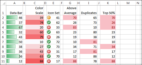
Figure 16.1. Visualizations such as data bars, color scales, icon sets, and top/bottom rules are controlled in the Excel user interface from the Conditional Formatting drop-down on the Home tab of the Ribbon.
VBA Methods and Properties for Data Visualizations
All the data visualization settings are managed in VBA with the FormatConditions collection. Conditional formatting has been in Excel since Excel 97. In Excel 2007, Microsoft expanded the FormatConditions object to handle the new visualizations. Whereas legacy versions of Excel would use the FormatConditions.Add method, Excel 2007–2013 offers additional methods such as AddDataBar, AddIconSetCondition, AddColorScale, AddTop10, AddAboveAverage, and AddUniqueValues.
It is possible to apply several different conditional formatting conditions to the same range. For example, you can apply a two-color color scale, an icon set, and a data bar to the same range. Excel includes a Priority property to specify which conditions should be calculated first. Methods such as SetFirstPriority and SetLastPriority ensure that a new format condition is executed before or after all others.
The StopIfTrue property works in conjunction with the Priority property. Say that you are highlighting duplicates but only want to check text cells. Create a new formula-based condition that use =ISNUMBER() to find numeric values. Make the ISNUMBER condition have a higher priority and apply StopIfTrue to prevent Excel from ever reaching the duplicates condition for numeric cells.
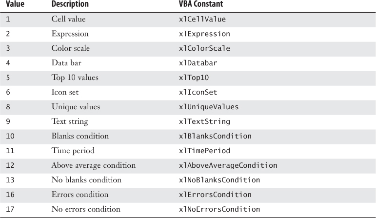
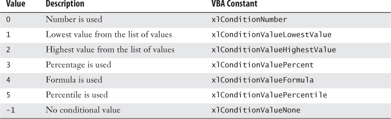
Beginning with Excel 2007, the Type property was expanded dramatically. This property was formerly a toggle between CellValue and Expression, but 13 new types were added in Excel 2007. Table 16.1 shows the valid values for the Type property. Items 3 and above were introduced in Excel 2007. The Excel team must have had plans for mode conditions; items 7, 14, and 15 do not exist, indicating they must have been on the drawing board at one time but then removed in the final version of Excel 2007. One of these was likely the ill-fated “highlight entire table row” feature that was in the Excel 2007 beta but removed in the final version.
Table 16.1. Valid Types for a Format Condition
Adding Data Bars to a Range
The Data Bar command adds an in-cell bar chart to each cell in a range. Many charting experts complained to Microsoft about problems in the Excel 2007 data bars. For this reason, Microsoft changed the data bars in Excel 2013 to address these problems.
In Figure 16.2, Cell C37 reflects changes introduced in Excel 2010. Notice that this cell, which has a value of 0, has no data bar at all. In Excel 2007, the smallest value receives a four-pixel data bar, even if that smallest value is 0. In addition, in Excel 2013 the largest bar in the dataset typically takes up the entire width of the cell.
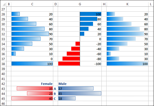
Figure 16.2. Excel 2013 offers many variations on data bars.
In Excel 2007, the data bars would end in a gradient that made it difficult to tell where the bar ended. Excel 2010–2013 offers a border around the bar. You can choose to change the color of the border or even to remove the border, as shown in Column K of the figure.
Excel 2010–2013 also offers support for negative data bars, as shown in Column G and the data bars that run right to left as shown in Cells C43:C45 of Figure 16.2. These allow comparative histograms.
Note
Although all of these are fine improvements, they add complexity to the VBA that is required to create data bars. In addition, you run the risk that your code will use new properties that will be incompatible with Excel 2007.
To add a data bar, you apply the .FormatConditions.AddDataBar method to a range containing your numbers. This method requires no arguments, and it returns an object of the DataBar type.
After you add the data bar, you will most likely need to change some of its properties. One method of referring to the data bar is to assume that the recently added data bar is the last item in the collection of format conditions. This code would add a data bar, identify the data bar by counting the conditions, and then change the color:
Range("A2:A11").FormatConditions.AddDatabar
ThisCond = Range("A2:A11").FormatConditions.Count
With Range("A2:A11").FormatConditions(ThisCond).BarColor
.Color = RGB(255, 0, 0) ' Red
.TintAndShade = -0.5 ' Darker than normal
End With
A safer way to go is to define an object variable of type DataBar. You can then assign the newly created data bar to the variable:
Dim DB As Databar
' Add the data bars
Set DB = Range("A2:A11").FormatConditions.AddDatabar
' Use a red that is 25% darker
With DB.BarColor
.Color = RGB(255, 0, 0)
.TintAndShade = -0.25
End With
When specifying colors for the data bar or the border, you should use the RGB function to assign a color. You can modify the color by making it darker or lighter using the TintAndShade property. Valid values are from -1 to 1. A value of 0 means no modification. Positive values make the color lighter. Negative values make the color darker.
By default, Excel assigns the shortest data bar to the minimum value and the longest data bar to the maximum value. If you want to override the defaults, use the Modify method for either the MinPoint or the MaxPoint properties. Specify a type from those shown in Table 16.2. Types 0, 3, 4, and 5 require a value. Table 16.2 shows valid types.
Table 16.2. MinPoint and MaxPoint Types
Use the following code to have the smallest bar assigned to values of 0 and below:
DB.MinPoint.Modify _
Newtype:=xlConditionValueNumber, NewValue:=0
To have the top 20 percent of the bars have the largest bar, use this code:
DB.MaxPoint.Modify _
Newtype:=xlConditionValuePercent, NewValue:=80
An interesting alternative is to show only the data bars and not the value. To do this, use this code:
DB.ShowValue = False
To show negative data bars in Excel 2013, use this line:
DB.AxisPosition = xlDataBarAxisAutomatic
When you allow negative data bars, you can specify an axis color, a negative bar color, and a negative bar border color. Samples of how to change the various colors are shown in the following code that creates the data bars shown in Column C of Figure 16.3:
Sub DataBar2()
' Add a Data bar
' Include negative data bars
' Control the min and max point
'
Dim DB As Databar
With Range("C2:C11")
.FormatConditions.Delete
' Add the data bars
Set DB = .FormatConditions.AddDatabar()
End With
' Set the lower limit
DB.MinPoint.Modify newtype:=xlConditionFormula, NewValue:="-600"
DB.MaxPoint.Modify newtype:=xlConditionValueFormula, NewValue:="600"
' Change the data bar to Green
With DB.BarColor
.Color = RGB(0, 255, 0)
.TintAndShade = -0.15
End With
' All of this is new in Excel 2010
With DB
' Use a gradient
.BarFillType = xlDataBarFillGradient
' Left to Right for direction of bars
.Direction = xlLTR
' Assign a different color to negative bars
.NegativeBarFormat.ColorType = xlDataBarColor
' Use a border around the bars
.BarBorder.Type = xlDataBarBorderSolid
' Assign a different border color to negative
.NegativeBarFormat.BorderColorType = xlDataBarSameAsPositive
' All borders are solid black
With .BarBorder.Color
.Color = RGB(0, 0, 0)
End With
' Axis where it naturally would fall, in black
.AxisPosition = xlDataBarAxisAutomatic
With .AxisColor
.Color = 0
.TintAndShade = 0
End With
' Negative bars in red
With .NegativeBarFormat.Color
.Color = 255
.TintAndShade = 0
End With
' Negative borders in red
End With
End Sub
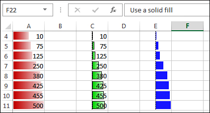
Figure 16.3. Data bars created by the macros in this section.
In Excel 2013, you have a choice of showing a gradient or a solid bar. To show a solid bar, use the following:
DB.BarFillType = xlDataBarFillSolid
The following code sample produces the solid bars shown in Column E of Figure 16.3:
Sub DataBar3()
' Add a Data bar
' Show solid bars
' Allow negative bars
' hide the numbers, show only the data bars
'
Dim DB As Databar
With Range("E2:E11")
.FormatConditions.Delete
' Add the data bars
Set DB = .FormatConditions.AddDatabar()
End With
With DB.BarColor
.Color = RGB(0, 0, 255)
.TintAndShade = 0.1
End With
' Hide the numbers
DB.ShowValue = False
' New in Excel 2013
DB.BarFillType = xlDataBarFillSolid
DB.NegativeBarFormat.ColorType = xlDataBarColor
With DB.NegativeBarFormat.Color
.Color = 255
.TintAndShade = 0
End With
' Allow negatives
DB.AxisPosition = xlDataBarAxisAutomatic
' Negative border color is different
DB.NegativeBarFormat.BorderColorType = xlDataBarColor
With DB.NegativeBarFormat.BorderColor
.Color = RGB(127, 127, 0)
.TintAndShade = 0
End With
End Sub
To allow the bars to go right to left, use this code:
DB.Direction = xlRTL ' Right to Left
Adding Color Scales to a Range
You can add color scales in either two-color or three-color scale varieties. Figure 16.4 shows the available settings in the Excel user interface for a color scale using three colors.
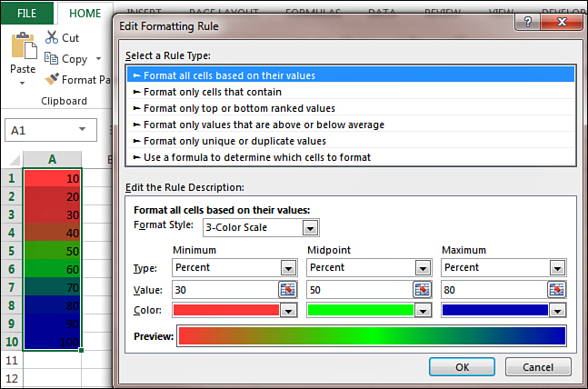
Figure 16.4. Color scales enable you to show hot spots in your dataset.
Like the data bar, you apply a color scale to a range object using the AddColorScale method. You should specify a ColorScaleType of either 2 or 3 as the only argument of the AddColorScale method.
Next, you can indicate a color and tint for both or all three of the color scale criteria. You can also specify whether the shade is applied to the lowest value, the highest value, a particular value, a percentage, or at a percentile using the values shown previously in Table 16.2.
The following code generates a three-color color scale in Range A1:A10:
Sub Add3ColorScale()
Dim CS As ColorScale
With Range("A1:A10")
.FormatConditions.Delete
' Add the Color Scale as a 3-color scale
Set CS = .FormatConditions.AddColorScale(ColorScaleType:=3)
End With
' Format the first color as light red
CS.ColorScaleCriteria(1).Type = xlConditionValuePercent
CS.ColorScaleCriteria(1).Value = 30
CS.ColorScaleCriteria(1).FormatColor.Color = RGB(255, 0, 0)
CS.ColorScaleCriteria(1).FormatColor.TintAndShade = 0.25
' Format the second color as green at 50%
CS.ColorScaleCriteria(2).Type = xlConditionValuePercent
CS.ColorScaleCriteria(2).Value = 50
CS.ColorScaleCriteria(2).FormatColor.Color = RGB(0, 255, 0)
CS.ColorScaleCriteria(2).FormatColor.TintAndShade = 0
' Format the third color as dark blue
CS.ColorScaleCriteria(3).Type = xlConditionValuePercent
CS.ColorScaleCriteria(3).Value = 80
CS.ColorScaleCriteria(3).FormatColor.Color = RGB(0, 0, 255)
CS.ColorScaleCriteria(3).FormatColor.TintAndShade = -0.25
End Sub
Adding Icon Sets to a Range
Icon sets in Excel come with three, four, or five different icons in the set. Figure 16.5 shows the settings for an icon set with five different icons.
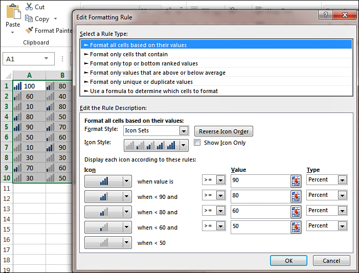
Figure 16.5. With additional icons, the complexity of the code increases.
To add an icon set to a range, use the AddIconSet method. No arguments are required. You can then adjust three properties that apply to the icon set. You then use several additional lines of code to specify the icon set in use and the limits for each icon.
Specifying an Icon Set
After adding the icon set, you can control whether the icon order is reversed, and whether Excel shows only the icons, and then specify one of the 20 built-in icon sets:
Dim ICS As IconSetCondition
With Range("A1:C10")
.FormatConditions.Delete
Set ICS = .FormatConditions.AddIconSetCondition()
End With
' Global settings for the icon set
With ICS
.ReverseOrder = False
.ShowIconOnly = False
.IconSet = ActiveWorkbook.IconSets(xl5CRV)
End With
Note
It is somewhat curious that the IconSets collection is a property of the active workbook. This seems to indicate that in future versions of Excel, new icon sets might be available.
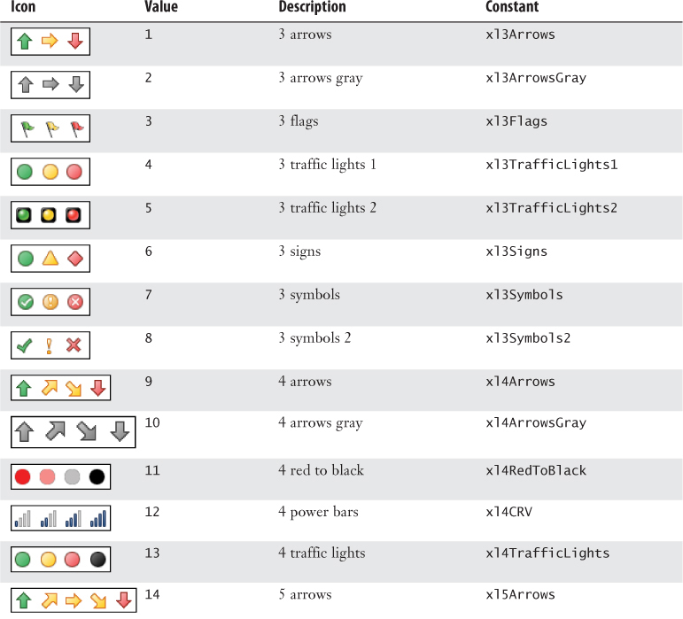
Table 16.3 shows the complete list of icon sets.
Table 16.3. Available Icon Sets and Their VBA Constants
Specifying Ranges for Each Icon
After specifying the type of icon set, you can specify ranges for each icon within the set. By default, the first icon starts at the lowest value. You can adjust the settings for each of the additional icons in the set:
' The first icon always starts at 0
' Settings for the second icon - start at 50%
With ICS.IconCriteria(2)
.Type = xlConditionValuePercent
.Value = 50
.Operator = xlGreaterEqual
End With
With ICS.IconCriteria(3)
.Type = xlConditionValuePercent
.Value = 60
.Operator = xlGreaterEqual
End With
With ICS.IconCriteria(4)
.Type = xlConditionValuePercent
.Value = 80
.Operator = xlGreaterEqual
End With
With ICS.IconCriteria(5)
.Type = xlConditionValuePercent
.Value = 90
.Operator = xlGreaterEqual
End With
Valid values for the Operator property are XlGreater or xlGreaterEqual.
Caution
With VBA, it is easy to create overlapping ranges such as icon 1 from 0 to 50 and icon 2 from 30 to 90. Even though the Edit Formatting Rule dialog box prevents overlapping ranges, VBA allows them. However, keep in mind that your icon set will display unpredictably if you create invalid ranges.
Using Visualization Tricks
If you use an icon set or a color scale, Excel applies a color to all cells in the dataset. Two tricks in this section enable you to apply an icon set to only a subset of the cells or to apply two different color data bars to the same range. The first trick is available in the user interface, but the second trick is available only in VBA.
Creating an Icon Set for a Subset of a Range
Sometimes, you might want to apply only a red X to the bad cells in a range. This is tricky to do in the user interface.
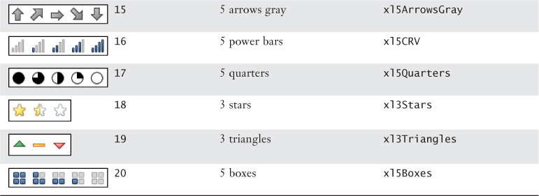
In the user interface, follow these steps to apply a red X to values greater than or equal to 80:
1. Add a three-symbols icon set to the range.
2. Specify that the symbols should be reversed.
3. Indicate that the red X icon appears for values greater than 80 (see Figure 16.6).
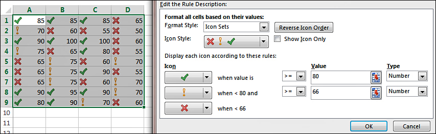
Figure 16.6. Add a three-icon set, paying particular attention to the value for the red X.
4. Open the drop-down next to the second icon. Choose No Cell Icon.
5. Open the drop-down next to the third icon. Choose No Cell Icon (see Figure 16.7).
Figure 16.7. Change the second and third rule to No Cell Icon.
The code to create this effect in VBA is straightforward. A great deal of the code is spent making sure that the icon set has the red X symbols on the cells greater than or equal to 80. To hide the icons for rules two and three, set the .Icon property to xlIconNoCellIcon.
The code to highlight values greater than or equal to 80 with a red X is shown here:
Sub TrickyFormatting()
' mark the bad cells
Dim ICS As IconSetCondition
Dim FC As FormatCondition
With Range("A1:D9")
.FormatConditions.Delete
Set ICS = .FormatConditions.AddIconSetCondition()
End With
With ICS
.ReverseOrder = True
.ShowIconOnly = False
.IconSet = ActiveWorkbook.IconSets(xl3Symbols2)
End With
' The threshhold for this icon doesn't really matter,
' but you have to make sure that it does not overlap the 3rd icon
With ICS.IconCriteria(2)
.Type = xlConditionValue
.Value = 66
.Operator = xlGreater
.Icon = xlIconNoCellIcon
End With
' Make sure the red X appears for cells 80 and above
With ICS.IconCriteria(3)
.Type = xlConditionValue
.Value = 80
.Operator = xlGreaterEqual
.Icon = xlIconNoCellIcon
End With
End Sub
Using Two Colors of Data Bars in a Range
This trick is particularly cool because it can be achieved only with VBA. Say that values greater than 90 are acceptable and those 90 and below indicate trouble. You would like acceptable values to have a green bar and others to have a red bar.
Using VBA, you first add the green data bars. Then, without deleting the format condition, you add red data bars.
In VBA, every format condition has a Formula property that defines whether the condition is displayed for a given cell. Therefore, the trick is to write a formula that defines when the green bars are displayed. When the formula is not True, the red bars are allowed to show through.
In Figure 16.8, the effect is being applied to Range A1:D10. You need to write the formula in A1 style, as if it applies to the top-left corner of the selection. The formula needs to evaluate to True or False. Excel automatically copies the formula to all the cells in the range. The formula for this condition is =IF(A1>90,True,False).
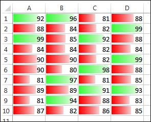
Figure 16.8. The dark bars are red, and the lighter bars are green. VBA was used to create two overlapping data bars, and then the Formula property hid the top bars for cells 90 and below.
Note
The formula is evaluated relative to the current cell pointer location. Even though it is not usually necessary to select cells before adding a FormatCondition, in this case, selecting the range ensures that the formula will work.
The following code creates the two-color data bars:
Sub AddTwoDataBars()
' passing values in green, failing in red
Dim DB As Databar
Dim DB2 As Databar
With Range("A1:D10")
.FormatConditions.Delete
' Add a Light Green Data Bar
Set DB = .FormatConditions.AddDatabar()
DB.BarColor.Color = RGB(0, 255, 0)
DB.BarColor.TintAndShade = 0.25
' Add a Red Data Bar
Set DB2 = .FormatConditions.AddDatabar()
DB2.BarColor.Color = RGB(255, 0, 0)
' Make the green bars only
.Select ' Required to make the next line work
.FormatConditions(1).Formula = "=IF(A1>90,True,False)"
DB.Formula = "=IF(A1>90,True,False)"
DB.MinPoint.Modify newtype:=xlConditionFormula, NewValue:="60"
DB.MaxPoint.Modify newtype:=xlConditionValueFormula, NewValue:="100"
DB2.MinPoint.Modify newtype:=xlConditionFormula, NewValue:="60"
DB2.MaxPoint.Modify newtype:=xlConditionValueFormula, NewValue:="100"
End With
End Sub
The Formula property works for all the conditional formats, which means you could potentially create some obnoxious combinations of data visualizations. In Figure 16.9, five different icon sets are combined in a single range. No one will be able to figure out whether a red flag is worse than a gray down arrow. Even so, this ability opens interesting combinations for those with a little creativity.
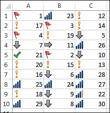
Figure 16.9. VBA created this mixture of five different icon sets in a single range. The Formula property in VBA is the key to combining icon sets.
Sub AddCrazyIcons()
With Range("A1:C10")
.Select ' The .Formula lines below require .Select here
.FormatConditions.Delete
' First icon set
.FormatConditions.AddIconSetCondition
.FormatConditions(1).IconSet = ActiveWorkbook.IconSets(xl3Flags)
.FormatConditions(1).Formula = "=IF(A1<5,TRUE,FALSE)"
' Next icon set
.FormatConditions.AddIconSetCondition
.FormatConditions(2).IconSet = ActiveWorkbook.IconSets(xl3ArrowsGray)
.FormatConditions(2).Formula = "=IF(A1<12,TRUE,FALSE)"
' Next icon set
.FormatConditions.AddIconSetCondition
.FormatConditions(3).IconSet = ActiveWorkbook.IconSets(xl3Symbols2)
.FormatConditions(3).Formula = "=IF(A1<22,TRUE,FALSE)"
' Next icon set
.FormatConditions.AddIconSetCondition
.FormatConditions(4).IconSet = ActiveWorkbook.IconSets(xl4CRV)
.FormatConditions(4).Formula = "=IF(A1<27,TRUE,FALSE)"
' Next icon set
.FormatConditions.AddIconSetCondition
.FormatConditions(5).IconSet = ActiveWorkbook.IconSets(xl5CRV)
End With
End Sub
Using Other Conditional Formatting Methods
Although the icon sets, data bars, and color scales get most of the attention, there are still plenty of other uses for conditional formatting.
The remaining examples in this chapter show some of the prior conditional formatting rules and some of the new methods available.
Formatting Cells That Are Above or Below Average
Use the AddAboveAverage method to format cells that are above or below average. After adding the conditional format, specify whether the AboveBelow property is xlAboveAverage or xlBelowAverage.
The following two macros highlight cells above and below average:
Sub FormatAboveAverage()
With Selection
.FormatConditions.Delete
.FormatConditions.AddAboveAverage
.FormatConditions(1).AboveBelow = xlAboveAverage
.FormatConditions(1).Interior.Color = RGB(255, 0, 0)
End With
End Sub
Sub FormatBelowAverage()
With Selection
.FormatConditions.Delete
.FormatConditions.AddAboveAverage
.FormatConditions(1).AboveBelow = xlBelowAverage
.FormatConditions(1).Interior.Color = RGB(255, 0, 0)
End With
End Sub
Formatting Cells in the Top 10 or Bottom 5
Four of the choices on the Top/Bottom Rules fly-out menu are controlled with the AddTop10 method. After you add the format condition, you need to set three properties that control how the condition is calculated:
• TopBottom—Set this to either xlTop10Top or xlTop10Bottom.
• Rank—Set this to 5 for the top 5, 6 for the top 6, and so on.
• Percent—Set this to False if you want the top 10 items. Set this to True if you want the top 10 percent of the items.
The following code highlights top or bottom cells:
Sub FormatTop10Items()
With Selection
.FormatConditions.Delete
.FormatConditions.AddTop10
.FormatConditions(1).TopBottom = xlTop10Top
.FormatConditions(1).Rank = 10
.FormatConditions(1).Percent = False
.FormatConditions(1).Interior.Color = RGB(255, 0, 0)
End With
End Sub
Sub FormatBottom5Items()
With Selection
.FormatConditions.Delete
.FormatConditions.AddTop10
.FormatConditions(1).TopBottom = xlTop10Bottom
.FormatConditions(1).Rank = 5
.FormatConditions(1).Percent = False
.FormatConditions(1).Interior.Color = RGB(255, 0, 0)
End With
End Sub
Sub FormatTop12Percent()
With Selection
.FormatConditions.Delete
.FormatConditions.AddTop10
.FormatConditions(1).TopBottom = xlTop10Top
.FormatConditions(1).Rank = 12
.FormatConditions(1).Percent = True
.FormatConditions(1).Interior.Color = RGB(255, 0, 0)
End With
End Sub
Formatting Unique or Duplicate Cells
The Remove Duplicates command on the Data tab of the Ribbon is a destructive command. You might want to mark the duplicates without removing them. If so, the AddUniqueValues method marks the duplicate or unique cells.
After calling the method, set the DupeUnique property to either xlUnique or xlDuplicate.
As I rant about in Excel 2013 In Depth (Que, ISBN 978-0-7897-4857-7), I do not really like either of these options. Choosing duplicate values marks both cells that contain the duplicate, as shown in Column A of Figure 16.10. For example, both A2 and A8 are marked, when A8 is really the only duplicate value.
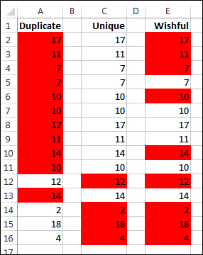
Figure 16.10. The AddUnique Values method can mark cells such as those in Columns A and C. Unfortunately, it cannot mark the truly useful pattern in Column E.
Choosing unique values marks only the cells that do not have a duplicate, as shown in Column C of Figure 16.10. This leaves several cells unmarked. For example, none of the cells containing 17 is marked.
As any data analyst knows, the truly useful option would have been to mark the first unique value. In this wishful state, Excel would mark one instance of each unique value. In this case, the 17 in E2 would be marked, but any subsequent cells that contain 17, such as E8, would remain unmarked.
The code to mark duplicates or unique values is shown here:
Sub FormatDuplicate()
With Selection
.FormatConditions.Delete
.FormatConditions.AddUniqueValues
.FormatConditions(1).DupeUnique = xlDuplicate
.FormatConditions(1).Interior.Color = RGB(255, 0, 0)
End With
End Sub
Sub FormatUnique()
With Selection
.FormatConditions.Delete
.FormatConditions.AddUniqueValues
.FormatConditions(1).DupeUnique = xlUnique
.FormatConditions(1).Interior.Color = RGB(255, 0, 0)
End With
End Sub
Sub HighlightFirstUnique()
With Range("E2:E16")
.Select
.FormatConditions.Delete
.FormatConditions.Add Type:=xlExpression, _
Formula1:="=COUNTIF(E$2:E2,E2)=1"
.FormatConditions(1).Interior.Color = RGB(255, 0, 0)
End With
End Sub
Formatting Cells Based on Their Value
The value conditional formats have been around for several versions of Excel. Use the Add method with the following arguments:
• Type—In this section, the type is xlCellValue.
• Operator—This can be xlBetween, xlEqual, xlGreater, xlGreaterEqual, xlLess, xlLessEqual, xlNotBetween, or xlNotEqual.
• Formula1—Formula1 is used with each of the operators specified to provide a numeric value.
• Formula2—This is used for xlBetween and xlNotBetween.
The following code sample highlights cells based on their values:
Sub FormatBetween10And20()
With Selection
.FormatConditions.Delete
.FormatConditions.Add Type:=xlCellValue, Operator:=xlBetween, _
Formula1:="=10", Formula2:="=20"
.FormatConditions(1).Interior.Color = RGB(255, 0, 0)
End With
End Sub
Sub FormatLessThan15()
With Selection
.FormatConditions.Delete
.FormatConditions.Add Type:=xlCellValue, Operator:=xlLess, _
Formula1:="=15"
.FormatConditions(1).Interior.Color = RGB(255, 0, 0)
End With
End Sub
Formatting Cells That Contain Text
When you are trying to highlight cells that contain a certain bit of text, you use the Add method, the xlTextString type, and an operator of xlBeginsWith, xlContains, xlDoesNotContain, or xlEndsWith.
The following code highlights all cells that contain a capital or lower case letter A:
Sub FormatContainsA()
With Selection
.FormatConditions.Delete
.FormatConditions.Add Type:=xlTextString, String:="A", _
TextOperator:=xlContains
' other choices: xlBeginsWith, xlDoesNotContain, xlEndsWith
.FormatConditions(1).Interior.Color = RGB(255, 0, 0)
End With
End Sub
Formatting Cells That Contain Dates
The date conditional formats were new in Excel 2007. The list of available date operators is a subset of the date operators available in the new pivot table filters. Use the Add method, the xlTimePeriod type, and one of these DateOperator values: xlYesterday, xlToday, xlTomorrow, xlLastWeek, xlLast7Days, xlThisWeek, xlNextWeek, xlLastMonth, xlThisMonth, or xlNextMonth.
The following code highlights all dates in the past week:
Sub FormatDatesLastWeek()
With Selection
.FormatConditions.Delete
' DateOperator choices include xlYesterday, xlToday, xlTomorrow,
' xlLastWeek, xlThisWeek, xlNextWeek, xlLast7Days
' xlLastMonth, xlThisMonth, xlNextMonth,
.FormatConditions.Add Type:=xlTimePeriod, DateOperator:=xlLastWeek
.FormatConditions(1).Interior.Color = RGB(255, 0, 0)
End With
End Sub
Formatting Cells That Contain Blanks or Errors
Buried deep within the Excel interface are options to format cells that contain blanks, contain errors, do not contain blanks, or do not contain errors. If you use the macro recorder, Excel uses the complicated xlExpression version of conditional formatting. For example, to look for a blank, Excel tests to see whether the =LEN(TRIM(A1))=0. Instead, you can use any of these four self-explanatory types. You are not required to use any other arguments with these new types:
.FormatConditions.Add Type:=xlBlanksCondition
.FormatConditions.Add Type:=xlErrorsCondition
.FormatConditions.Add Type:=xlNoBlanksCondition
.FormatConditions.Add Type:=xlNoErrorsCondition
Using a Formula to Determine Which Cells to Format
The most powerful conditional format is still the xlExpression type. In this type, you provide a formula for the active cell that evaluates to True or False. Make sure to write the formula with relative or absolute references so that the formula is correct when Excel copies the formula to the remaining cells in the selection.
An infinite number of conditions can be identified with a formula. Two popular conditions are shown here.
Highlight the First Unique Occurrence of Each Value in a Range
In Column A of Figure 16.11, you would like to highlight the first occurrence of each value in the column. The highlighted cells will then contain a complete list of the unique numbers found in the column.
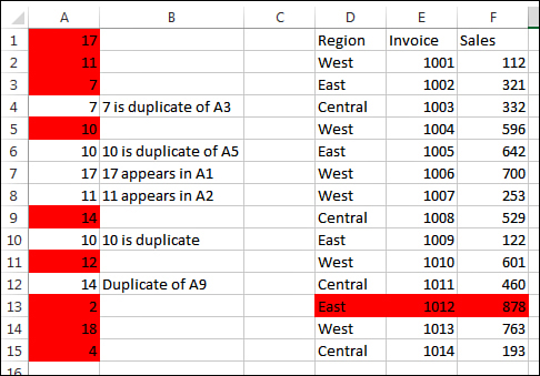
Figure 16.11. A formula-based condition can mark the first unique occurrence of each value, as shown in Column A, or the entire row with the largest sales, as shown in D:F.
The macro should select Cells A1:A15. The formula should be written to return a True or False value for Cell A1. Because Excel logically copies this formula to the entire range, you should use a careful combination of relative and absolute references.
The formula can use the COUNTIF function. Check to see how many times the range from A$1 to A1 contains the value A1. If the result is equal to 1, the condition is True and the cell is highlighted. The first formula is =COUNTIF(A$1:A1,A1)=1. As the formula is copied down to, say A12, the formula changes to =COUNTIF(A$1:A12,A12)=1.
The following macro creates the formatting shown in Column A of Figure 16.11:
Sub HighlightFirstUnique()
With Range("A1:A15")
.Select
.FormatConditions.Delete
.FormatConditions.Add Type:=xlExpression, _
Formula1:="=COUNTIF(A$1:A1,A1)=1"
.FormatConditions(1).Interior.Color = RGB(255, 0, 0)
End With
End Sub
Highlight the Entire Row for the Largest Sales Value
Another example of a formula-based condition is when you want to highlight the entire row of a dataset in response to a value in one column. Consider the dataset in Cells D2:F15 of Figure 16.11. If you want to highlight the entire row that contains the largest sale, you select Cells D2:F15 and write a formula that works for Cell D2: =$F2=MAX($F$2:$F$15). The code required to format the row with the largest sales value is as follows:
Sub HighlightWholeRow()
With Range("D2:F15")
.Select
.FormatConditions.Delete
.FormatConditions.Add Type:=xlExpression, _
Formula1:="=$F2=MAX($F$2:$F$15)"
.FormatConditions(1).Interior.Color = RGB(255, 0, 0)
End With
End Sub
Using the New NumberFormat Property
In legacy versions of Excel, a cell that matched a conditional format could have a particular font, font color, border, or fill pattern. As of Excel 2007, you can also specify a number format. This can prove useful for selectively changing the number format used to display the values.
For example, you might want to display numbers greater than 999 in thousands, numbers greater than 999,999 in hundred thousands, and numbers greater than 9 million in millions.
If you turn on the macro recorder and attempt to record setting the conditional format to a custom number format, the Excel 2013 VBA macro recorder actually records the action of executing an XL4 macro! Skip the recorded code and use the NumberFormat property as shown here:
Sub NumberFormat()
With Range("E1:G26")
.FormatConditions.Delete
.FormatConditions.Add Type:=xlCellValue, Operator:=xlGreater, _
Formula1:="=9999999"
.FormatConditions(1).NumberFormat = "$#,##0,""M"""
.FormatConditions.Add Type:=xlCellValue, Operator:=xlGreater,
Formula1:="=999999"
.FormatConditions(2).NumberFormat = "$#,##0.0,""M"""
.FormatConditions.Add Type:=xlCellValue, Operator:=xlGreater,
Formula1:="=999"
.FormatConditions(3).NumberFormat = "$#,##0,K"
End With
End Sub
Figure 16.12 shows the original numbers in Columns A:C. The results of running the macro are shown in Columns E:G. The dialog box shows the resulting conditional format rules.
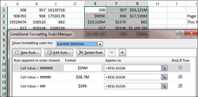
Figure 16.12. Since Excel 2007, conditional formats have been able to specify a specific number format.
Next Steps
In Chapter 17, you’ll find out how to create dashboards from tiny charts called sparklines.