13. Excel Power

A major secret of successful programmers is to never waste time writing the same code twice. They all have little bits—or even big bits—of code that they use over and over again. Another big secret is to never take 8 hours doing something that can be done in 10 minutes—which is what this book is about!

This chapter contains programs donated by several Excel power programmers. These are programs they have found useful, and they hope these will help you too. Not only can these programs save you time, but they also can teach you new ways of solving common problems.

Different programmers have different programming styles, and we did not rewrite the submissions. As you review the lines of code, you will notice different ways of doing the same task, such as referring to ranges.

File Operations

The following utilities deal with handling files in folders. Being able to loop through a list of files in a folder is a useful task.

List Files in a Directory

Submitted by our good friend Nathan P. Oliver of Minneapolis, Minnesota.

This program returns the filename, size, and date modified of all specified file types in the selected directory and its subfolders:

Sub ExcelFileSearch()
Dim srchExt As Variant, srchDir As Variant
Dim i As Long, j As Long, strName As String
Dim varArr(1 To 1048576, 1 To 3) As Variant
Dim strFileFullName As String
Dim ws As Worksheet
Dim fso As Object

Let srchExt = Application.InputBox("Please Enter File Extension", "Info Request")
If srchExt = False And Not TypeName(srchExt) = "String" Then
    Exit Sub
End If

Let srchDir = BrowseForFolderShell
If srchDir = False And Not TypeName(srchDir) = "String" Then
    Exit Sub
End If

Application.ScreenUpdating = False

Set ws = ThisWorkbook.Worksheets.Add(Sheets(1))
On Error Resume Next
Application.DisplayAlerts = False
ThisWorkbook.Worksheets("FileSearch Results").Delete
Application.DisplayAlerts = True
On Error GoTo 0
ws.Name = "FileSearch Results"

Let strName = Dir$(srchDir & "*" & srchExt)
Do While strName <> vbNullString
    Let i = i + 1
    Let strFileFullName = srchDir & strName
    Let varArr(i, 1) = strFileFullName
    Let varArr(i, 2) = FileLen(strFileFullName) 1024
    Let varArr(i, 3) = FileDateTime(strFileFullName)
    Let strName = Dir$()
Loop

Set fso = CreateObject("Scripting.FileSystemObject")
Call recurseSubFolders(fso.GetFolder(srchDir), varArr(), i, CStr(srchExt))
Set fso = Nothing

ThisWorkbook.Windows(1).DisplayHeadings = False
With ws
    If i > 0 Then
        .Range("A2").Resize(i, UBound(varArr, 2)).Value = varArr
        For j = 1 To i
            .Hyperlinks.Add anchor:=.Cells(j + 1, 1), Address:=varArr(j, 1)
        Next
    End If
    .Range(.Cells(1, 4), .Cells(1, .Columns.Count)).EntireColumn.Hidden = True
    .Range(.Cells(.Rows.Count, 1).End(xlUp)(2), _
        .Cells(.Rows.Count, 1)).EntireRow.Hidden = True
    With .Range("A1:C1")
        .Value = Array("Full Name", "Kilobytes", "Last Modified")
        .Font.Underline = xlUnderlineStyleSingle
        .EntireColumn.AutoFit
        .HorizontalAlignment = xlCenter
    End With
End With
Application.ScreenUpdating = True
End Sub

Private Sub recurseSubFolders(ByRef Folder As Object, _
    ByRef varArr() As Variant, _
    ByRef i As Long, _
    ByRef srchExt As String)
Dim SubFolder As Object
Dim strName As String, strFileFullName As String
For Each SubFolder In Folder.SubFolders
    Let strName = Dir$(SubFolder.Path & "*" & srchExt)
    Do While strName <> vbNullString
        Let i = i + 1
        Let strFileFullName = SubFolder.Path & "" & strName
        Let varArr(i, 1) = strFileFullName
        Let varArr(i, 2) = FileLen(strFileFullName) 1024
        Let varArr(i, 3) = FileDateTime(strFileFullName)
        Let strName = Dir$()
    Loop
    If i > 1048576 Then Exit Sub
    Call recurseSubFolders(SubFolder, varArr(), i, srchExt)
Next
End Sub

Private Function BrowseForFolderShell() As Variant
Dim objShell As Object, objFolder As Object
Set objShell = CreateObject("Shell.Application")
Set objFolder = objShell.BrowseForFolder(0, "Please select a folder", 0, "C:")
If Not objFolder Is Nothing Then
    On Error Resume Next
    If IsError(objFolder.Items.Item.Path) Then
        BrowseForFolderShell = CStr(objFolder)
    Else
        On Error GoTo 0
        If Len(objFolder.Items.Item.Path) > 3 Then
            BrowseForFolderShell = objFolder.Items.Item.Path & _
            Application.PathSeparator
        Else
            BrowseForFolderShell = objFolder.Items.Item.Path
        End If
    End If
Else
    BrowseForFolderShell = False
End If
Set objFolder = Nothing: Set objShell = Nothing
End Function

Import CSV

Submitted by Masaru Kaji of Kobe-City, Japan. Masaru is a computer system’s administrator. He maintains an Excel VBA tip site, Colo’s Excel Junk Room, at excel.toypark.in/tips.shtml

If you find yourself importing a lot of comma-separated variable (CSV) files and then having to go back and delete them, this program is for you. It quickly opens a CSV in Excel and permanently deletes the original file.

Option Base 1

Sub OpenLargeCSVFast()
    Dim buf(1 To 16384) As Variant
    Dim i As Long
    'Change the file location and name here
    Const strFilePath As String = "C: empSales.CSV"

    Dim strRenamedPath As String
    strRenamedPath = Split(strFilePath, ".")(0) & "txt"

    With Application
        .ScreenUpdating = False
        .DisplayAlerts = False
    End With
    'Setting an array for FieldInfo to open CSV
    For i = 1 To 16384
        buf(i) = Array(i, 2)
    Next
    Name strFilePath As strRenamedPath
    Workbooks.OpenText Filename:=strRenamedPath, DataType:=xlDelimited, _
                       Comma:=True, FieldInfo:=buf
    Erase buf
    ActiveSheet.UsedRange.Copy ThisWorkbook.Sheets(1).Range("A1")
    ActiveWorkbook.Close False
    Kill strRenamedPath
    With Application
        .ScreenUpdating = True
        .DisplayAlerts = True
    End With
End Sub

Read Entire TXT to Memory and Parse

Submitted by Suat Mehmet Ozgur of Istanbul, Turkey. Suat develops applications in Excel, Access, and Visual Basic.

This sample takes a different approach to reading a text file. Instead of reading one record at a time, the macro loads the entire text file into memory in a single string variable. The macro then parses the string into individual records. The advantage of this method is that you access the file on disk only one time. All subsequent processing occurs in memory and is very fast.

Sub ReadTxtLines()
'No need to install Scripting Runtime library since we used late binding
Dim sht As Worksheet
Dim fso As Object
Dim fil As Object
Dim txt As Object
Dim strtxt As String
Dim tmpLoc As Long

    'Working on active sheet
    Set sht = ActiveSheet
    'Clear data in the sheet
   sht.UsedRange.ClearContents

    'File system object that we need to manage files
    Set fso = CreateObject("Scripting.FileSystemObject")

    'File that we like to open and read
    Set fil = fso.GetFile("c: empSales.txt")

    'Opening file as a TextStream
    Set txt = fil.OpenAsTextStream(1)

    'Reading entire file into a string variable at once
    strtxt = txt.ReadAll

    'Close textstream and free the file. We don't need it anymore.
    txt.Close

    'Find the first placement of new line char
    tmpLoc = InStr(1, strtxt, vbCrLf)

    'Loop until no more new line
    Do Until tmpLoc = 0
        'Use A column and next empty cell to write the text file line
        sht.Cells(sht.Rows.Count, 1).End(xlUp).Offset(1).Value = _
            Left(strtxt, tmpLoc - 1)

        'Remove the parsed line from the variable where we stored the entire file
        strtxt = Right(strtxt, Len(strtxt) - tmpLoc - 1)

        'Find the next placement of new line char
        tmpLoc = InStr(1, strtxt, vbCrLf)
    Loop

    'Last line that has data but no new line char
    sht.Cells(sht.Rows.Count, 1).End(xlUp).Offset(1).Value = strtxt

    'It will be already released by the ending of this procedure but
    ' as a good habit, set the object as nothing.
    Set fso = Nothing
End Sub

Combining and Separating Workbooks

The next four utilities demonstrate how to combine worksheets into a single workbook or separate a single workbook into individual worksheets or Word documents.

Separate Worksheets into Workbooks

Submitted by Tommy Miles of Houston, Texas.

This sample goes through the active workbook and saves each sheet as its own workbook in the same path as the original workbook. It names the new workbooks based on the sheet name, and it overwrites files without prompting. You will also notice that you need to choose whether you save the file as XLSM (macro-enabled) or XLSX (macros will be stripped). In the following code, both lines are included—xlsm and xlsx—but the xlsx lines are commented out, making them inactive:

Sub SplitWorkbook()

Dim ws As Worksheet
Dim DisplayStatusBar As Boolean

DisplayStatusBar = Application.DisplayStatusBar
Application.DisplayStatusBar = True
Application.ScreenUpdating = False
Application.DisplayAlerts = False

For Each ws In ThisWorkbook.Sheets
    Dim NewFileName As String
    Application.StatusBar = ThisWorkbook.Sheets.Count & " Remaining Sheets"
    If ThisWorkbook.Sheets.Count <> 1 Then
        NewFileName = ThisWorkbook.Path & "" & ws.Name & ".xlsm" 'Macro-Enabled
'       NewFileName = ThisWorkbook.Path & "" & ws.Name & ".xlsx" _
           'Not Macro-Enabled
        ws.Copy
        ActiveWorkbook.Sheets(1).Name = "Sheet1"
        ActiveWorkbook.SaveAs Filename:=NewFileName, _
            FileFormat:=xlOpenXMLWorkbookMacroEnabled
'        ActiveWorkbook.SaveAs Filename:=NewFileName, _
            FileFormat:=xlOpenXMLWorkbook
        ActiveWorkbook.Close SaveChanges:=False
    Else
        NewFileName = ThisWorkbook.Path & "" & ws.Name & ".xlsm"
'        NewFileName = ThisWorkbook.Path & "" & ws.Name & ".xlsx"
        ws.Name = "Sheet1"
    End If
Next

Application.DisplayAlerts = True
Application.StatusBar = False
Application.DisplayStatusBar = DisplayStatusBar
Application.ScreenUpdating = True
End Sub

Combine Workbooks

Submitted by Tommy Miles.

This sample goes through all the Excel files in a specified directory and combines them into a single workbook. It renames the sheets based on the name of the original workbook.

Sub CombineWorkbooks()
    Dim CurFile As String, DirLoc As String
    Dim DestWB As Workbook
    Dim ws As Object 'allows for different sheet types

    DirLoc = ThisWorkbook.Path & " st" 'location of files
    CurFile = Dir(DirLoc & "*.xls*")

    Application.ScreenUpdating = False
    Application.EnableEvents = False

    Set DestWB = Workbooks.Add(xlWorksheet)

    Do While CurFile <> vbNullString
        Dim OrigWB As Workbook
        Set OrigWB = Workbooks.Open(Filename:=DirLoc & CurFile, ReadOnly:=True)

        ' Limit to valid sheet names and removes .xls*
        CurFile = Left(Left(CurFile, Len(CurFile) - 5), 29)

        For Each ws In OrigWB.Sheets
            ws.Copy After:=DestWB.Sheets(DestWB.Sheets.Count)

            If OrigWB.Sheets.Count > 1 Then
                DestWB.Sheets(DestWB.Sheets.Count).Name = CurFile & ws.Index
            Else
                DestWB.Sheets(DestWB.Sheets.Count).Name = CurFile
            End If
        Next

        OrigWB.Close SaveChanges:=False
        CurFile = Dir
    Loop

    Application.DisplayAlerts = False
    DestWB.Sheets(1).Delete
    Application.DisplayAlerts = True

    Application.ScreenUpdating = True
    Application.EnableEvents = True

    Set DestWB = Nothing
End Sub

Filter and Copy Data to Separate Worksheets

Submitted by Dennis Wallentin of Ostersund, Sweden. Dennis provides Excel tips and tricks at http://xldennis.wordpress.com/.

This sample uses a specified column to filter data and copies the results to new worksheets in the active workbook:

Sub Filter_NewSheet()
Dim wbBook As Workbook
Dim wsSheet As Worksheet
Dim rnStart As Range, rnData As Range
Dim i As Long

Set wbBook = ThisWorkbook
Set wsSheet = wbBook.Worksheets("Sheet1")

With wsSheet
    'Make sure that the first row contains headings.
    Set rnStart = .Range("A2")
    Set rnData = .Range(.Range("A2"), .Cells(.Rows.Count, 3).End(xlUp))
End With

Application.ScreenUpdating = True

For i = 1 To 5
    'Here we filter the data with the first criterion.
    rnStart.AutoFilter Field:=1, Criteria1:="AA" & i
    'Copy the filtered list
    rnData.SpecialCells(xlCellTypeVisible).Copy
    'Add a new worksheet to the active workbook.
    Worksheets.Add Before:=wsSheet
    'Name the added new worksheets.
    ActiveSheet.Name = "AA" & i
    'Paste the filtered list.
    Range("A2").PasteSpecial xlPasteValues
Next i

'Reset the list to its original status.
rnStart.AutoFilter Field:=1

With Application
    'Reset the clipboard.
    .CutCopyMode = False
    .ScreenUpdating = False
End With

End Sub

Export Data to Word

Submitted by Dennis Wallentin.

This program transfers data from Excel to the first table found in a Word document. It uses early binding, so a reference must be established in the VB Editor using Tools, References to the Microsoft Word object library.

Sub Export_Data_Word_Table()
Dim wdApp As Word.Application
Dim wdDoc As Word.Document
Dim wdCell As Word.Cell
Dim i As Long
Dim wbBook As Workbook
Dim wsSheet As Worksheet
Dim rnData As Range
Dim vaData As Variant

Set wbBook = ThisWorkbook
Set wsSheet = wbBook.Worksheets("Sheet1")

With wsSheet
    Set rnData = .Range("A1:A10")
End With

'Add the values in the range to a one-dimensional variant-array.
vaData = rnData.Value

'Here we instantiate the new object.
Set wdApp = New Word.Application
'Here the target document resides in the same folder as the workbook.
Set wdDoc = wdApp.Documents.Open(ThisWorkbook.Path & "Test.docx")

'Import data to the first table and in the first column of a ten-row table.
For Each wdCell In wdDoc.Tables(1).Columns(1).Cells
    i = i + 1
    wdCell.Range.Text = vaData(i, 1)
Next wdCell

'Save and close the document.
With wdDoc
    .Save
    .Close
End With

'Close the hidden instance of Microsoft Word.
wdApp.Quit
'Release the external variables from the memory
Set wdDoc = Nothing
Set wdApp = Nothing

MsgBox "The data has been transferred to Test.docx.", vbInformation

End Sub

Working with Cell Comments

Cell comments are often underused features of Excel. The following three utilities help you get the most out of cell comments.

List Comments

Submitted by Tommy Miles.

Excel allows the user to print the comments in a workbook; however, it does not specify the workbook or worksheet on which the comments appear, but only the cell, as shown in Figure 13.1.

Figure 13.1. Excel prints only the origin cell address and its comment.

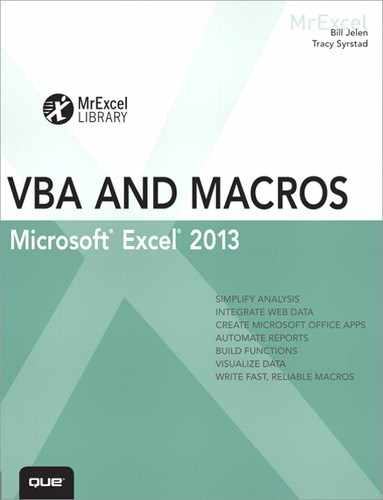
The following sample places comments, author, and location of each comment on a new sheet for easy viewing, saving, or printing. Figure 13.2 shows a sample result.

Sub ListComments()
    Dim wb As Workbook
    Dim ws As Worksheet

    Dim cmt As Comment

    Dim cmtCount As Long

    cmtCount = 2

    On Error Resume Next
        Set ws = ActiveSheet
            If ws Is Nothing Then Exit Sub
    On Error GoTo 0

    Application.ScreenUpdating = False

    Set wb = Workbooks.Add(xlWorksheet)

    With wb.Sheets(1)
        .Range("$A$1") = "Author"
        .Range("$B$1") = "Book"
        .Range("$C$1") = "Sheet"
        .Range("$D$1") = "Range"
        .Range("$E$1") = "Comment"
    End With

    For Each cmt In ws.Comments
        With wb.Sheets(1)
            .Cells(cmtCount, 1) = cmt.author
'Parent is the object to which another object belongs.
'For example, the parent of a comment is the cell in which it resides.
'The parent of the cell is the sheet on which it resides.
'So if you have Comment.Parent.Parent.Name, you are returning the sheet name.
            .Cells(cmtCount, 2) = cmt.Parent.Parent.Parent.Name
            .Cells(cmtCount, 3) = cmt.Parent.Parent.Name
            .Cells(cmtCount, 4) = cmt.Parent.Address
            .Cells(cmtCount, 5) = CleanComment(cmt.author, cmt.Text)
        End With

        cmtCount = cmtCount + 1
    Next

    wb.Sheets(1).UsedRange.WrapText = False

    Application.ScreenUpdating = True

    Set ws = Nothing
    Set wb = Nothing
End Sub

Private Function CleanComment(author As String, cmt As String) As String
    Dim tmp As String

    tmp = Application.WorksheetFunction.Substitute(cmt, author & ":", "")
    tmp = Application.WorksheetFunction.Substitute(tmp, Chr(10), "")

    CleanComment = tmp
End Function

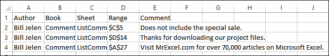
Figure 13.2. Easily list all the information pertaining to comments.

Resize Comments

Submitted by Tom Urtis of San Francisco, California. Tom is the principal owner of Atlas Programming Management, an Excel consulting firm in the Bay Area.

Excel doesn’t automatically resize cell comments. In addition, if you have several on a sheet, as shown in Figure 13.3, it can be a hassle to resize them one at a time. The following sample code resizes all the comment boxes on a sheet so that, when selected, the entire comment is easily viewable, as shown in Figure 13.4.

Sub CommentFitter1()
Application.ScreenUpdating = False
Dim x As Range, y As Long

For Each x In Cells.SpecialCells(xlCellTypeComments)
    Select Case True
        Case Len(x.NoteText) <> 0
            With x.Comment
                .Shape.TextFrame.AutoSize = True
                If .Shape.Width > 250 Then
                    y = .Shape.Width * .Shape.Height
                    .Shape.Width = 150
                    .Shape.Height = (y / 200) * 1.3
                End If
            End With
    End Select
Next x
Application.ScreenUpdating = True
End Sub

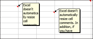
Figure 13.3. By default, Excel doesn’t size the comment boxes to show all the entered text.

Figure 13.4. Resize the comment boxes to fit all the text.

Place a Chart in a Comment

Submitted by Tom Urtis.

A live chart cannot exist in a shape, but you can take a picture of the chart and load it into the comment shape, as shown in Figure 13.5.

Figure 13.5. Place a chart in a cell comment.

The steps to do this manually are as given here:

1. Create and save the picture image you want the comment to display.

2. If you have not already done so, create the comment and select the cell in which the comment is located.

3. From the Review tab, select Edit Comment, or right-click the cell and select Edit Comment.

4. Right-click the comment border and select Format Comment.

5. Select the Colors and Lines tab, and click the down arrow belonging to the Color field of the Fill section.

6. Select Fill Effects, select the Picture tab, and then click the Select Picture button.

7. Navigate to your desired image, select the image, and click OK twice.

The effect of having a “live chart” in a comment can be achieved if, for example, the code is part of a SheetChange event when the chart’s source data is being changed. In addition, business charts are updated often, so you might want a macro to keep the comment updated and to avoid repeating the same steps.

The following macro does just that—just modify the macro for file pathname, chart name, destination sheet, cell, and size of comment shape, depending on the size of the chart:

Sub PlaceGraph()
Dim x As String, z As Range

Application.ScreenUpdating = False

'assign a temporary location to hold the image
x = "C: empXWMJGraph.gif"

'assign the cell to hold the comment
Set z = Worksheets("ChartInComment").Range("A3")

'delete any existing comment in the cell
On Error Resume Next
z.Comment.Delete
On Error GoTo 0

'select and export the chart
ActiveSheet.ChartObjects("Chart 1").Activate
ActiveChart.Export x

'add a new comment to the cell, set the size and insert the chart
With z.AddComment
    With .Shape
        .Height = 322
        .Width = 465
        .Fill.UserPicture x
    End With
End With

'delete the temporary image
Kill x

Range("A1").Activate
Application.ScreenUpdating = True

Set z = Nothing
End Sub

Utilities to Wow Your Clients

The next four utilities will amaze and impress your clients.

Using Conditional Formatting to Highlight Selected Cell

Submitted by Ivan F. Moala of Auckland, New Zealand. Ivan is the site author of The XcelFiles (www.xcelfiles.com), where you can find out how to do things you thought you could not do in Excel.

Conditional formatting is used to highlight the row and column of the active cell to help you visually locate it, as shown in Figure 13.6.

Figure 13.6. Use conditional formatting to highlight the selected cell in a table.

Const iInternational As Integer = Not (0)

Private Sub Worksheet_SelectionChange(ByVal Target As Range)
Dim iColor As Integer
'// On error resume in case
'// user selects a range of cells
On Error Resume Next
iColor = Target.Interior.ColorIndex
'// Leave On Error ON for Row offset errors

If iColor < 0 Then
    iColor = 36
Else
    iColor = iColor + 1
End If

'// Need this test in case font color is the same
If iColor = Target.Font.ColorIndex Then iColor = iColor + 1

Cells.FormatConditions.Delete

'// Horizontal color banding
With Range("A" & Target.Row, Target.Address) 'Rows(Target.Row)
    .FormatConditions.Add Type:=2, Formula1:=iInternational 'Or just 1 '"TRUE"
    .FormatConditions(1).Interior.ColorIndex = iColor
End With

'// Vertical color banding
With Range(Target.Offset(1 - Target.Row, 0).Address & ":" & _
    Target.Offset(-1, 0).Address)
    .FormatConditions.Add Type:=2, Formula1:=iInternational 'Or just 1 '"TRUE"
    .FormatConditions(1).Interior.ColorIndex = iColor
End With

End Sub

Highlight Selected Cell Without Using Conditional Formatting

Submitted by Ivan F. Moala.

This example visually highlights the active cell without using conditional formatting when the keyboard arrow keys are used to move around the sheet.

Place the following in a standard module:

Dim strCol As String
Dim iCol As Integer
Dim dblRow As Double

Sub HighlightRight()
    HighLight 0, 1
End Sub

Sub HighlightLeft()
    HighLight 0, -1
End Sub

Sub HighlightUp()
    HighLight -1, 0, -1
End Sub

Sub HighlightDown()
    HighLight 1, 0, 1
End Sub

Sub HighLight(dblxRow As Double, iyCol As Integer, Optional dblZ As Double = 0)
On Error GoTo NoGo
strCol = Mid(ActiveCell.Offset(dblxRow, iyCol).Address, _
        InStr(ActiveCell.Offset(dblxRow, iyCol).Address, "$") + 1, _
        InStr(2, ActiveCell.Offset(dblxRow, iyCol).Address, "$") - 2)
iCol = ActiveCell.Column
dblRow = ActiveCell.Row

Application.ScreenUpdating = False

With Range(strCol & ":" & strCol & "," & dblRow + dblZ & ":" & dblRow + dblZ)
    .Select
    Application.ScreenUpdating = True
    .Item(dblRow + dblxRow).Activate
End With

NoGo:
End Sub

Sub ReSet() 'manual reset
    Application.OnKey "{RIGHT}"
    Application.OnKey "{LEFT}"
    Application.OnKey "{UP}"
    Application.OnKey "{DOWN}"
End Sub

Place the following in the ThisWorkbook module:

Private Sub Workbook_Open()
    Application.OnKey "{RIGHT}", "HighlightRight"
    Application.OnKey "{LEFT}", "HighlightLeft"
    Application.OnKey "{UP}", "HighlightUp"
    Application.OnKey "{DOWN}", "HighlightDown"
    Application.OnKey "{DEL}", "DisableDelete"
End Sub

Private Sub Workbook_BeforeClose(Cancel As Boolean)
    Application.OnKey "{RIGHT}"
    Application.OnKey "{LEFT}"
    Application.OnKey "{UP}"
    Application.OnKey "{DOWN}"
    Application.OnKey "{DEL}"
End Sub

Custom Transpose Data

Submitted by Masaru Kaji.

You have a report where the data is set up in rows (see Figure 13.7). However, you need the data formatted such that each date and batch is in a single row, with the Value and Finish Position going across. Note that the Finish Position is not shown in Figure 13.8. The following program does a customized data transposition based on the specified column, as shown in Figure 13.8.

Sub TransposeData()
Dim shOrg As Worksheet, shRes As Worksheet
Dim rngStart As Range, rngPaste As Range
Dim lngData As Long

Application.ScreenUpdating = False
On Error Resume Next
Application.DisplayAlerts = False
Sheets("TransposeResult").Delete
Application.DisplayAlerts = True
On Error GoTo 0

On Error GoTo terminate

Set shOrg = Sheets("TransposeData")
Set shRes = Sheets.Add(After:=shOrg)
shRes.Name = "TransposeResult"
With shOrg
    '--Sort
    .Cells.CurrentRegion.Sort Key1:=.[B2], Order1:=1, Key2:=.[C2], _
       Order2:=1, Key3:=.[E2], Order3:=1, Header:=xlYes
    '--Copy title
    .Rows(1).Copy shRes.Rows(1)
    '--Set start range
    Set rngStart = .[C2]
    Do Until IsEmpty(rngStart)
        Set rngPaste = shRes.Cells(shRes.Rows.Count, 1).End(xlUp).Offset(1)
        lngData = GetNextRange(rngStart)
        rngStart.Offset(, -2).Resize(, 5).Copy rngPaste

        'Copy to V1 to V14
        rngStart.Offset(, 2).Resize(lngData).Copy
        rngPaste.Offset(, 5).PasteSpecial Paste:=xlAll, Operation:=xlNone, _
         SkipBlanks:=False, Transpose:=True
        'Copy to V1FP to V14FP
        rngStart.Offset(, 1).Resize(lngData).Copy
        rngPaste.Offset(, 19).PasteSpecial Paste:=xlAll, Operation:=xlNone, _
         SkipBlanks:=False, Transpose:=True
        Set rngStart = rngStart.Offset(lngData)
    Loop
End With

Application.Goto shRes.[A1]
With shRes
    .Cells.Columns.AutoFit
    .Columns("D:E").Delete shift:=xlToLeft
End With

Application.ScreenUpdating = True
Application.CutCopyMode = False

If MsgBox("Do you want to delete the original worksheet?", 36) = 6 Then
'6 is the numerical value of vbYes
    Application.DisplayAlerts = False
    Sheets("TransposeData").Delete
    Application.DisplayAlerts = True
End If

Set rngPaste = Nothing
Set rngStart = Nothing
Set shRes = Nothing

Exit Sub

terminate:
End Sub

Function GetNextRange(ByVal rngSt As Range) As Long
    Dim i As Long
    i = 0

    Do Until rngSt.Value <> rngSt.Offset(i).Value
        i = i + 1
    Loop

    GetNextRange = i
End Function

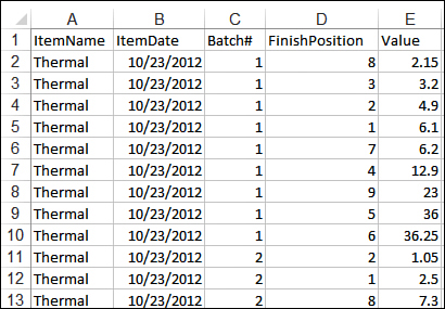
Figure 13.7. The original data has similar records in separate rows.

Figure 13.8. The formatted data transposes the data so that identical dates and batches are merged into a single row.

Select/Deselect Noncontiguous Cells

Submitted by Tom Urtis.

Ordinarily, to deselect a single cell or range on a sheet, you must click an unselected cell to deselect all cells and then start over by reselecting all the correct cells. This is inconvenient if you need to reselect a lot of noncontiguous cells.

This sample adds two new options to the contextual menu of a selection: Deselect ActiveCell and Deselect ActiveArea. With the noncontiguous cells selected, hold down the Ctrl key, click the cell you want to deselect to make it active, release the Ctrl key, and then right-click the cell you want to deselect. The contextual menu shown in Figure 13.9 appears. Click the menu item that deselects either that one active cell or the contiguously selected area of which it is a part.

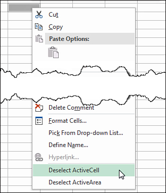
Figure 13.9. The Modify RightClick procedure provides a custom contextual menu for deselecting noncontiguous cells.

Enter the following procedures in a standard module:

Sub ModifyRightClick()
'add the new options to the right-click menu
Dim O1 As Object, O2 As Object

'delete the options if they exist already
On Error Resume Next
With CommandBars("Cell")
    .Controls("Deselect ActiveCell").Delete
    .Controls("Deselect ActiveArea").Delete
End With
On Error GoTo 0

'add the new options
Set O1 = CommandBars("Cell").Controls.Add

With O1
    .Caption = "Deselect ActiveCell"
    .OnAction = "DeselectActiveCell"
End With

Set O2 = CommandBars("Cell").Controls.Add

With O2
    .Caption = "Deselect ActiveArea"
    .OnAction = "DeselectActiveArea"
End With
End Sub

Sub DeselectActiveCell()
Dim x As Range, y As Range

If Selection.Cells.Count > 1 Then
    For Each y In Selection.Cells
        If y.Address <> ActiveCell.Address Then
            If x Is Nothing Then
                Set x = y
            Else
                Set x = Application.Union(x, y)
            End If
        End If
    Next y
    If x.Cells.Count > 0 Then
        x.Select
    End If
End If
End Sub

Sub DeselectActiveArea()
Dim x As Range, y As Range

If Selection.Areas.Count > 1 Then
    For Each y In Selection.Areas
        If Application.Intersect(ActiveCell, y) Is Nothing Then
            If x Is Nothing Then
                Set x = y
            Else
                Set x = Application.Union(x, y)
            End If
        End If
    Next y
    x.Select
End If
End Sub

Add the following procedures to the ThisWorkbook module:

Private Sub Workbook_Activate()
ModifyRightClick
End Sub

Private Sub Workbook_Deactivate()
Application.CommandBars("Cell").Reset
End Sub

Techniques for VBA Pros

The next eight utilities amaze me. In the various message board communities on the Internet, VBA programmers are constantly coming up with new ways to do something faster or better. When someone posts some new code that obviously runs circles around the prior generally accepted best code, everyone benefits.

Excel State Class Module

Submitted by Juan Pablo Gonzàlez Ruiz of Bogotà, Colombia. Juan Pablo is an Excel consultant and runs his photography business at www.juanpg.com.

The following class module is one of my favorites and I use it in almost every project I create. Before Juan shared the module with me, I used to enter the four lines of code to turn off and back on screen updating, events, alerts, and calculations. At the beginning of a sub I would turn them off, and at the end I would turn them back on. That was quite a bit of typing. Now, I just place the class module in a new workbook I create and call it as needed.

Insert a class module named CAppState and place the following code in it:

Private m_su As Boolean
Private m_ee As Boolean
Private m_da As Boolean
Private m_calc As Long
Private m_cursor As Long

Private m_except As StateEnum

Public Enum StateEnum
    None = 0
    ScreenUpdating = 1
    EnableEvents = 2
    DisplayAlerts = 4
    Calculation = 8
    Cursor = 16
End Enum

Public Sub SetState(Optional ByVal except As StateEnum = StateEnum.None)
    m_except = except
    With Application
        If Not m_except And StateEnum.ScreenUpdating Then
            .ScreenUpdating = False
        End If

        If Not m_except And StateEnum.EnableEvents Then
            .EnableEvents = False
        End If

        If Not m_except And StateEnum.DisplayAlerts Then
            .DisplayAlerts = False
        End If

        If Not m_except And StateEnum.Calculation Then
            .Calculation = xlCalculationManual
        End If

        If Not m_except And StateEnum.Cursor Then
            .Cursor = xlWait
        End If
    End With
End Sub

Private Sub Class_Initialize()
    With Application
        m_su = .ScreenUpdating
        m_ee = .EnableEvents
        m_da = .DisplayAlerts
        m_calc = .Calculation
        m_cursor = .Cursor
    End With
End Sub

Private Sub Class_Terminate()
    With Application
        If Not m_except And StateEnum.ScreenUpdating Then
            .ScreenUpdating = m_su
        End If

        If Not m_except And StateEnum.EnableEvents Then
            .EnableEvents = m_ee
        End If

        If Not m_except And StateEnum.DisplayAlerts Then
            .DisplayAlerts = m_da
        End If

        If Not m_except And StateEnum.Calculation Then
            .Calculation = m_calc
        End If

        If Not m_except And StateEnum.Cursor Then
            .Cursor = m_cursor
        End If
    End With
End Sub

The following code is an example of calling the class module to turn off the various states, running your code, and then setting the states back.

Sub RunFasterCode
Dim appState As CAppState
Set appState = New CAppState
appState.SetState None
'run your code
'if you have any formulas that need to update, use
'Application.Calculate
'to force the workbook to calculate
Set appState = Nothing
End Sub

Pivot Table Drill-Down

Submitted by Tom Urtis.

When you are double-clicking the data section, a pivot table’s default behavior is to insert a new worksheet and display that drill-down information on the new sheet. The following example serves as an option for convenience, to keep the drilled-down recordsets on the same sheet as the pivot table (see Figure 13.10) so that you can delete them as you want.

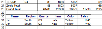
Figure 13.10. Show the drill-down recordset on the same sheet as the pivot table.

To use this macro, double-click the data section or the Totals section to create stacked drill-down recordsets in the next available row of the sheet. To delete any drill-down recordsets you have created, double-click anywhere in their respective current region.

Private Sub Worksheet_BeforeDoubleClick(ByVal Target As Range, Cancel As Boolean)
Application.ScreenUpdating = False
Dim LPTR&

With ActiveSheet.PivotTables(1).DataBodyRange
    LPTR = .Rows.Count + .Row - 1
End With

Dim PTT As Integer
On Error Resume Next
PTT = Target.PivotCell.PivotCellType
If Err.Number = 1004 Then
    Err.Clear
    If Not IsEmpty(Target) Then
        If Target.Row > Range("A1").CurrentRegion.Rows.Count + 1 Then
            Cancel = True
            With Target.CurrentRegion
                .Resize(.Rows.Count + 1).EntireRow.Delete
            End With
        End If
    Else
        Cancel = True
    End If
Else
    CS = ActiveSheet.Name
End If
Application.ScreenUpdating = True
End Sub

Custom Sort Order

Submitted by Wei Jiang of Wuhan City, China. Jiang is a consultant for MrExcel.com.

By default, Excel enables you to sort lists numerically or alphabetically, but sometimes that is not what is needed. For example, a client might need each day’s sales data sorted by the default division order of belts, handbags, watches, wallets, and everything else. Although you can manually set up a custom series and sort using it, if you’re creating an automated workbook for other users, this might not be an option. This sample uses a custom sort order list to sort a range of data into default division order and then deletes the custom sort order. Figure 13.11 shows the results.

Sub CustomSort()
    ' add the custom list to Custom Lists
    Application.AddCustomList ListArray:=Range("I1:I5")

    ' get the list number
    nIndex = Application.GetCustomListNum(Range("I1:I5").Value)

    ' Now, we could sort a range with the custom list.
    ' Note, we should use nIndex + 1 as the custom list number here,
    ' for the first one is Normal order
    Range("A2:C16").Sort Key1:=Range("B2"), Order1:=xlAscending, _
                            Header:=xlNo, Orientation:=xlSortColumns, _
                            OrderCustom:=nIndex + 1
    Range("A2:C16").Sort Key1:=Range("A2"), Order1:=xlAscending, _
                            Header:=xlNo, Orientation:=xlSortColumns

    ' At the end, we should remove this custom list...
    Application.DeleteCustomList nIndex
End Sub

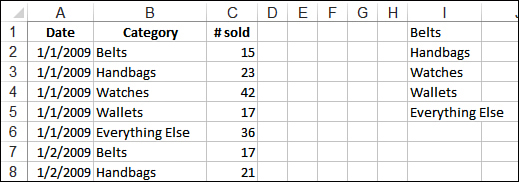
Figure 13.11. When you use the macro, the list in A:C is sorted first by date and then by the custom sort list in Column I.

Cell Progress Indicator

Submitted by Tom Urtis.

I have to admit, the conditional formatting options in Excel, such as data bars, are fantastic. However, there still isn’t an option for a visual like that shown in Figure 13.12. The following example builds a progress indicator in Column C based on entries in Columns A and B.

Private Sub Worksheet_Change(ByVal Target As Range)
If Target.Column > 2 Or Target.Cells.Count > 1 Then Exit Sub
If Application.IsNumber(Target.Value) = False Then
    Application.EnableEvents = False
    Application.Undo
    Application.EnableEvents = True
    MsgBox "Numbers only please."
    Exit Sub
End If
Select Case Target.Column
    Case 1
        If Target.Value > Target.Offset(0, 1).Value Then
            Application.EnableEvents = False
            Application.Undo
            Application.EnableEvents = True
            MsgBox "Value in column A may not be larger than value in column B."
            Exit Sub
        End If
    Case 2
        If Target.Value < Target.Offset(0, -1).Value Then
            Application.EnableEvents = False
            Application.Undo
            Application.EnableEvents = True
            MsgBox "Value in column B may not be smaller " & _
                "than value in column A."
            Exit Sub
        End If
End Select
Dim x As Long
x = Target.Row
Dim z As String
z = Range("B" & x).Value - Range("A" & x).Value
With Range("C" & x)
    .Formula = "=IF(RC[-1]<=RC[-2],REPT(""n"",RC[-1]) _
        &REPT(""n"",RC[-2]-RC[-1]),REPT(""n"",RC[-2]) _
        &REPT(""o"",RC[-1]-RC[-2]))"
    .Value = .Value
    .Font.Name = "Wingdings"
    .Font.ColorIndex = 1
    .Font.Size = 10
    If Len(Range("A" & x)) <> 0 Then
        .Characters(1, (.Characters.Count - z)).Font.ColorIndex = 3
        .Characters(1, (.Characters.Count - z)).Font.Size = 12
    End If
End With
End Sub

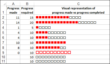
Figure 13.12. Use indicators in cells to show progress.

Protected Password Box

Submitted by Daniel Klann of Sydney, Australia. Daniel works mainly with VBA in Excel and Access, but dabbles in all sorts of languages.

Using an input box for password protection has a major security flaw: The characters being entered are easily viewable. This program changes the characters to asterisks as they are entered—just like a real password field (see Figure 13.13). Note that the code that follows does not work in 64-bit Excel. Refer to Chapter 23, “Windows Application Programming Interface (API),” for information on modifying the code for 64-bit Excel.

Private Declare Function CallNextHookEx Lib "user32" (ByVal hHook As Long, _
ByVal ncode As Long, ByVal wParam As Long, lParam As Any) As Long

Private Declare Function GetModuleHandle Lib "kernel32" _
    Alias "GetModuleHandleA" (ByVal lpModuleName As String) As Long

Private Declare Function SetWindowsHookEx Lib "user32" _
    Alias "SetWindowsHookExA" _
    (ByVal idHook As Long, ByVal lpfn As Long, _
    ByVal hmod As Long,ByVal dwThreadId As Long) As Long

Private Declare Function UnhookWindowsHookEx Lib "user32" _
    (ByVal hHook As Long) As Long

Private Declare Function SendDlgItemMessage Lib "user32" _
    Alias "SendDlgItemMessageA" _
    (ByVal hDlg As Long, _
    ByVal nIDDlgItem As Long, ByVal wMsg As Long, _
    ByVal wParam As Long, ByVal lParam As Long) As Long

Private Declare Function GetClassName Lib "user32" _
    Alias "GetClassNameA" (ByVal hwnd As Long, _
    ByVal lpClassName As String, _
    ByVal nMaxCount As Long) As Long

Private Declare Function GetCurrentThreadId _
    Lib "kernel32" () As Long

'Constants to be used in our API functions
Private Const EM_SETPASSWORDCHAR = &HCC
Private Const WH_CBT = 5
Private Const HCBT_ACTIVATE = 5
Private Const HC_ACTION = 0

Private hHook As Long

Public Function NewProc(ByVal lngCode As Long, _
    ByVal wParam As Long, ByVal lParam As Long) As Long
    Dim RetVal
    Dim strClassName As String, lngBuffer As Long

    If lngCode < HC_ACTION Then
        NewProc = CallNextHookEx(hHook, lngCode, wParam, lParam)
        Exit Function
    End If

    strClassName = String$(256, " ")
    lngBuffer = 255

    If lngCode = HCBT_ACTIVATE Then    'A window has been activated

        RetVal = GetClassName(wParam, strClassName, lngBuffer)

        'Check for class name of the Inputbox
        If Left$(strClassName, RetVal) = "#32770" Then
            'Change the edit control to display the password character *.
            'You can change the Asc("*") as you please.
            SendDlgItemMessage wParam, &H1324, EM_SETPASSWORDCHAR, Asc("*"), &H0
        End If

    End If

    'This line will ensure that any other hooks that may be in place are
    'called correctly.
    CallNextHookEx hHook, lngCode, wParam, lParam
End Function

Public Function InputBoxDK(Prompt, Optional Title, _
    Optional Default, Optional XPos, _
    Optional YPos, Optional HelpFile, Optional Context) As String
    Dim lngModHwnd As Long, lngThreadID As Long

    lngThreadID = GetCurrentThreadId
    lngModHwnd = GetModuleHandle(vbNullString)

    hHook = SetWindowsHookEx(WH_CBT, AddressOf NewProc, lngModHwnd, lngThreadID)
    On Error Resume Next
    InputBoxDK = InputBox(Prompt, Title, Default, XPos, YPos, HelpFile, Context)
    UnhookWindowsHookEx hHook
End Function

Sub PasswordBox()
If InputBoxDK("Please enter password", "Password Required") <> "password" Then

        MsgBox "Sorry, that was not a correct password."
    Else
        MsgBox "Correct Password!  Come on in."
    End If
End Sub

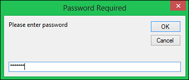
Figure 13.13. Use an input box as a secure password field.

Change Case

Submitted by Ivan F. Moala.

Word can change the case of selected text, but that capability is notably lacking in Excel. This program enables the Excel user to change the case of text in any selected range, as shown in Figure 13.14.

Sub TextCaseChange()
Dim RgText As Range
Dim oCell As Range
Dim Ans As String
Dim strTest As String
Dim sCap As Integer, _
    lCap As Integer, _
    i As Integer

'// You need to select a range to alter first!

Again:
Ans = Application.InputBox("[L]owercase" & vbCr & "[U]ppercase" & vbCr & _
        "[S]entence" & vbCr & "[T]itles" & vbCr & "[C]apsSmall", _
        "Type in a Letter", Type:=2)

If Ans = "False" Then Exit Sub
If InStr(1, "LUSTC", UCase(Ans), vbTextCompare) = 0 _
    Or Len(Ans) > 1 Then GoTo Again

On Error GoTo NoText
If Selection.Count = 1 Then
    Set RgText = Selection
Else
    Set RgText = Selection.SpecialCells(xlCellTypeConstants, 2)
End If
On Error GoTo 0

For Each oCell In RgText
    Select Case UCase(Ans)
        Case "L": oCell = LCase(oCell.Text)
        Case "U": oCell = UCase(oCell.Text)
        Case "S": oCell = UCase(Left(oCell.Text, 1)) & _
            LCase(Right(oCell.Text, Len(oCell.Text) - 1))
        Case "T": oCell = Application.WorksheetFunction.Proper(oCell.Text)
        Case "C"
                lCap = oCell.Characters(1, 1).Font.Size
                sCap = Int(lCap * 0.85)
                'Small caps for everything.
                oCell.Font.Size = sCap
                oCell.Value = UCase(oCell.Text)
                strTest = oCell.Value
                'Large caps for 1st letter of words.
                strTest = Application.Proper(strTest)
                For i = 1 To Len(strTest)
                    If Mid(strTest, i, 1) = UCase(Mid(strTest, i, 1)) Then
                        oCell.Characters(i, 1).Font.Size = lCap
                    End If
                Next i
    End Select
Next

Exit Sub
NoText:
MsgBox "No text in your selection @ " & Selection.Address

End Sub

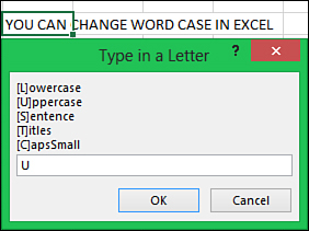
Figure 13.14. You can now change the case of words, just like in Word.

Selecting with SpecialCells

Submitted by Ivan F. Moala.

Typically, when you want to find certain values, text, or formulas in a range, the range is selected and each cell is tested. The following example shows how SpecialCells can be used to select only the desired cells. Having fewer cells to check speeds up your code.

The following code ran in the blink of an eye on my machine. However, the version that checked each cell in the range (A1:Z20000) took 14 seconds—an eternity in the automation world!

Sub SpecialRange()
Dim TheRange As Range
Dim oCell As Range

    Set TheRange = Range("A1:Z20000").SpecialCells(__
    xlCellTypeConstants, xlTextValues)

    For Each oCell In TheRange
        If oCell.Text = "Your Text" Then
            MsgBox oCell.Address
            MsgBox TheRange.Cells.Count
        End If
    Next oCell

End Sub

ActiveX Right-Click Menu

Submitted by Tom Urtis.

There is no built-in menu for the right-click event of ActiveX objects on a sheet. This is a utility for that, using a command button for the example in Figure 13.15. Set the Take Focus on Click property of the command button to False.

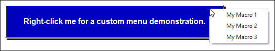
Figure 13.15. Customize the contextual (right-click) menu of an ActiveX control.

Place the following in the ThisWorkbook module:

Private Sub Workbook_Open()
With Application
    .CommandBars("Cell").Reset
    .WindowState = xlMaximized
    .Goto Sheet1.Range("A1"), True
End With
End Sub

Private Sub Workbook_Activate()
Application.CommandBars("Cell").Reset
End Sub

Private Sub Workbook_SheetBeforeRightClick(ByVal Sh As Object, _
   ByVal Target As Range, Cancel As Boolean)
Application.CommandBars("Cell").Reset
End Sub

Private Sub Workbook_Deactivate()
Application.CommandBars("Cell").Reset
End Sub

Private Sub Workbook_BeforeClose(Cancel As Boolean)
With Application
    .CommandBars("Cell").Reset
    .WindowState = xlMaximized
    .Goto Sheet1.Range("A1"), True
End With
ThisWorkbook.Save
End Sub

Place the following in the control’s sheet module, such as Sheet1:

Private Sub CommandButton1_Click()
MsgBox "You left-clicked the command button." & vbCrLf & _
"Right-click the button for a custom menu demonstration.", 64, "FYI..."
End Sub

Private Sub CommandButton1_MouseDown ()
If Button = 2 Then Run "MyRightClickMenu"
End Sub

Place the following in a standard module:

Sub MyRightClickMenu()
Application.CommandBars("Cell").Reset
Dim cbc As CommandBarControl
  For Each cbc In Application.CommandBars("cell").Controls
      cbc.Visible = False
  Next cbc
With Application.CommandBars("Cell").Controls.Add(temporary:=True)
    .Caption = "My Macro 1"
    .OnAction = "Test1"
   End With
With Application.CommandBars("Cell").Controls.Add(temporary:=True)
    .Caption = "My Macro 2"
    .OnAction = "Test2"
   End With
With Application.CommandBars("Cell").Controls.Add(temporary:=True)
    .Caption = "My Macro 3"
    .OnAction = "Test3"
   End With
Application.CommandBars("Cell").ShowPopup
End Sub

Sub Test1()
MsgBox "This is the Test1 macro from the ActiveX object's custom " & _
    "right-click event menu.", , "''My Macro 1'' menu item."
End Sub

Sub Test2()
MsgBox "This is the Test2 macro from the ActiveX object's custom " & _
    "right-click event menu.", , "''My Macro 2'' menu item."
End Sub

Sub Test3()
MsgBox "This is the Test3 macro from the ActiveX object's custom " & _
    "right-click event menu.", , "''My Macro 3'' menu item."
End Sub

Cool Applications

These last samples are interesting applications that you might be able to incorporate into your own projects.

Historical Stock/Fund Quotes

Submitted by Nathan P. Oliver.

The following code retrieves the average of a valid stock ticker or the close of a fund for the specified date:

Private Sub GetQuote()
Dim ie As Object, lCharPos As Long, sHTML As String
Dim HistDate As Date, HighVal As String, LowVal As String
Dim cl As Range

Set cl = ActiveCell
HistDate = cl(, 0)

If Intersect(cl, Range("C2:C" & Cells.Rows.Count)) Is Nothing Then
    MsgBox "You must select a cell in column C."
    Exit Sub
End If

If Not CBool(Len(cl(, -1))) Or Not CBool(Len(cl(, 0))) Then
    MsgBox "You must enter a symbol and date."
    Exit Sub
End If

Set ie = CreateObject("InternetExplorer.Application")

With ie
    .Navigate _
        "http://bigcharts.marketwatch.com/historical" & _
        "/default.asp?detect=1&symb=" _
        & cl(, -1) & "&closedate=" & Month(HistDate) & "%2F" & _
        Day(HistDate) & "%2F" & Year(HistDate) & "&x=0&y=0"
    Do While .Busy And .ReadyState <> 4
        DoEvents
    Loop
    sHTML = .Document.body.innertext
    .Quit
End With

Set ie = Nothing

lCharPos = InStr(1, sHTML, "High:", vbTextCompare)
If lCharPos Then HighVal = Mid$(sHTML, lCharPos + 5, 15)

If Not Left$(HighVal, 3) = "n/a" Then
    lCharPos = InStr(1, sHTML, "Low:", vbTextCompare)
    If lCharPos Then LowVal = Mid$(sHTML, lCharPos + 4, 15)
    cl.Value = (Val(LowVal) + Val(HighVal)) / 2
Else: lCharPos = InStr(1, sHTML, "Closing Price:", vbTextCompare)
    cl.Value = Val(Mid$(sHTML, lCharPos + 14, 15))
End If

Set cl = Nothing
End Sub

Using VBA Extensibility to Add Code to New Workbooks

You have a macro that moves data to a new workbook for the regional managers. What if you need to also copy macros to the new workbook? You can use Visual Basic for Application Extensibility to import modules to a workbook or to actually write lines of code to the workbook.

To use any of these examples, you must first open VB Editor, select References from the Tools menu, and select the reference for Microsoft Visual Basic for Applications Extensibility 5.3. You must also trust access to VBA by going to the Developer tab, choosing Macro Security, and checking Trust Access to the VBA Project Object Model.

The easiest way to use VBA Extensibility is to export a complete module or userform from the current project and import it to the new workbook. Perhaps you have an application with thousands of lines of code. You want to create a new workbook with data for the regional manager and give her three macros to enable custom formatting and printing. Place all of these macros in a module called modToRegion. Macros in this module also call the frmRegion userform. The following code transfers this code from the current workbook to the new workbook:

Sub MoveDataAndMacro()
    Dim WSD as worksheet
    Set WSD = Worksheets("Report")
    ' Copy Report to a new workbook
    WSD.Copy
    ' The active workbook is now the new workbook
    ' Delete any old copy of the module from C
    On Error Resume Next
    ' Delete any stray copies from hard drive
    Kill ("C: empModToRegion.bas")
    Kill ("C: empfrmRegion.frm")
    On Error GoTo 0
    ' Export module & form from this workbook
    ThisWorkbook.VBProject.VBComponents("ModToRegion").Export _
       ("C: empModToRegion.bas")
    ThisWorkbook.VBProject.VBComponents("frmRegion").Export _
       ("C: empfrmRegion. frm")
    ' Import to new workbook
    ActiveWorkbook.VBProject.VBComponents.Import ("C: empModToRegion.bas")
    ActiveWorkbook.VBProject.VBComponents.Import ("C: empfrmRegion.frm")
    On Error Resume Next
    Kill ("C: empModToRegion.bas")
    Kill ("C: empfrmRegion.bas")
    On Error GoTo 0
End Sub

The preceding method works if you need to move modules or userforms to a new workbook. However, what if you need to write some code to the Workbook_Open macro in the ThisWorkbook module? There are two tools to use. The Lines method enables you to return a particular set of code lines from a given module. The InsertLines method enables you to insert code lines to a new module.

Sub MoveDataAndMacro()
    Dim WSD as worksheet
    Dim WBN as Workbook
    Dim WBCodeMod1 As Object, WBCodeMod2 As Object
    Set WSD = Worksheets("Report")
    ' Copy Report to a new workbook
    WSD.Copy
    ' The active workbook is now the new workbook
    Set WBN = ActiveWorkbook
    ' Copy the Workbook level Event handlers
    Set WBCodeMod1 = ThisWorkbook.VBProject.VBComponents("ThisWorkbook") _
      .CodeModule
    Set WBCodeMod2 = WBN.VBProject.VBComponents("ThisWorkbook").CodeModule
    WBCodeMod2.insertlines 1, WBCodeMod1.Lines(1, WBCodeMod1.countoflines)
End Sub

Next Steps

The utilities in this chapter aren’t Excel’s only source of programming power. User-defined functions (UDFs) enable you to create complex custom formulas to cover what Excel’s functions don’t. In Chapter 14, “Sample User-Defined Functions,” you’ll find out how to create and share your own functions.