
Chapter 10 - Temporary Tables
“I cannot imagine any condition which would cause this ship to founder. Modern shipbuilding has gone beyond that.”
– E. I. Smith, Captain of the Titanic
There are Three types of Temporary Tables
Derived Table
Exists only within a query
Materialized by a SELECT Statement inside a query
Space comes from the User’s Spool space
Deleted when the query ends
Volatile Table
Created by the User and materialized with an INSERT/SELECT
Space comes from the User’s Spool space
Table and Data are deleted only after a User Logs off the session
Global Temporary Table
Table definition is created by a User and the table definition is permanent
Materialized with an INSERT/SELECT
Space comes from the User’s TEMP Space
When User logs off the session the data is deleted, but the table definition stays
Many Users can populate the same Global table, but each has their own copy
The three types of Temporary tables are Derived, Volatile and Global Temporary Tables.
CREATING A Derived Table
• Exists only within a query
• Materialized by a SELECT Statement inside a query
• Space comes from the User’s Spool space
• Deleted when the query ends

The SELECT Statement that creates and populates the Derived table is always inside Parentheses.
Naming the Derived Table
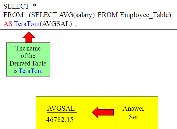
In the example above, TeraTom is the name we gave the Derived Table. It is mandatory that you always name the table or it errors.
Aliasing the Column Names in The Derived Table

AVGSAL is the name we gave to the column in our Derived Table that we call TeraTom. Our SELECT (which builds the columns) shows we are only going to have one column in our derived table, and we have named that column AVGSAL.
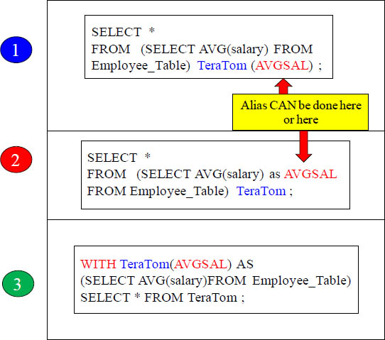
Multiple Ways to Alias the Columns in a Derived Table

CREATING A Derived Table using the WITH Command

When using the WITH Command, we can CREATE our Derived table before running the main query. The only issue here is that you can only have 1 WITH.
The Same Derived Query shown Three Different Ways
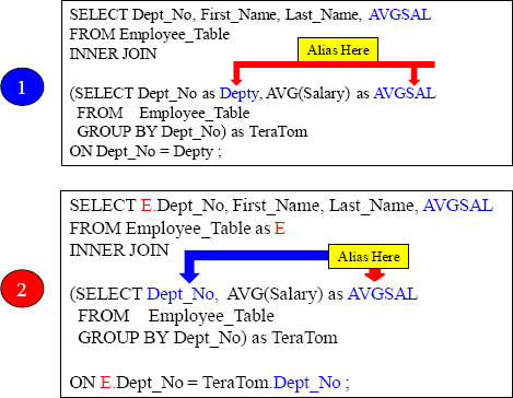
Most Derived Tables Are Used To Join To Other Tables

The first five columns in the Answer Set came from the Employee_Table. AVGSAL came from the derived table named TeraTom.
The Three Components of a Derived Table

|
A derived table will always have a SELECT query to materialize the derived table with data. The SELECT query always starts with an open parenthesis and ends with a close parenthesis. |
|
The derived table must be given a name. Above we called our derived table TeraTom. |
|
You will need to define (alias) the columns in the derived table. Above we allowed Dept_No to default to Dept_No, but we had to specifically alias AVG(Salary) as AVGSAL. |
Every derived table must have the three components listed above.
Visualize This Derived Table

Our example above shows the data in the derived table named TeraTom. This query allows us to see each employee and the plus or minus avg of their salary compared to the other workers in their department.
Our Join Example With A Different Column Aliasing Style

Column Aliasing Can Default For Normal Columns

TeraTom |
|
Dept_No |
AVGSAL |
? |
32800.50 |
10 |
64300.00 |
100 |
48850.00 |
200 |
44944.44 |
300 |
40200.00 |
400 |
48333.33 |
The derived table |
|
In a derived table, you will always have a SELECT query in parenthesis, and you will always name the table. You have options when aliasing the columns. As in the example above, you can let normal columns default to their current name.
Our Join Example With The WITH Syntax

Now, the lower portion of the query refers to TeraTom Almost like it is a permanent table, but it is not!
Quiz - Answer the Questions
SELECT Dept_No, First_Name, Last_Name, AVGSAL
FROM Employee_Table
INNER JOIN
(SELECT Dept_No, AVG(Salary)
FROM Employee_Table
GROUP BY Dept_No) as TeraTom (Depty, AVGSAL)
ON Dept_No = Depty ;
1) What is the name of the derived table? __________
2) How many columns are in the derived table? _______
3) What is the name of the derived table columns? ______
4) Is there more than one row in the derived table? _______
5) What common keys join the Employee and Derived? _______
6) Why were the join keys named differently? ______________
Answer to Quiz - Answer the Questions
SELECT Dept_No, First_Name, Last_Name, AVGSAL
FROM Employee_Table
INNER JOIN
(SELECT Dept_No, AVG(Salary)
FROM Employee_Table
GROUP BY Dept_No) as TeraTom (Depty, AVGSAL)
ON Dept_No = Depty ;
1) What is the name of the derived table? TeraTom
2) How many columns are in the derived table? 2
3) What’s the name of the derived columns? Depty and AVGSAL
4) Is their more than one row in the derived table? Yes
5) What keys join the tables? Dept_No and Depty
6) Why were the join keys named differently? If both were named Dept_No, we would error unless we full qualified.
Clever Tricks on Aliasing Columns in a Derived Table
A Derived Table lives only for the lifetime of a single query
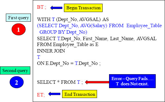
An Example of Two Derived Tables in a Single Query
WITH T (Dept_No, AVGSAL) AS
(SELECT Dept_No, AVG(Salary) FROM Employee_Table
GROUP BY Dept_No)
SELECT T.Dept_No, First_Name, Last_Name,
AVGSAL, Counter
FROM Employee_Table as E
INNER JOIN
T
ON E.Dept_No = T.Dept_No
INNER JOIN
(SELECT Employee_No, SUM(1) OVER(PARTITION BY Dept_No ORDER BY Dept_No, Last_Name Rows Unbounded Preceding)
FROM Employee_Table) as S (Employee_No, Counter)
ON E.Employee_No = S.Employee_No
ORDER BY T.Dept_No;
WITH RECURSIVE Derived Table Hierarchy

Above is a company hierarchy and this is what we will use to perform our WITH Recursive query.
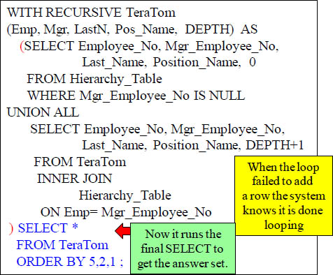
WITH RECURSIVE Derived Table Query
WITH RECURSIVE TeraTom
(Emp, Mgr, LastN, Pos_Name, DEPTH) AS
(SELECT Employee_No, Mgr_Employee_No,
Last_Name, Position_Name, 0
FROM Hierarchy_Table
WHERE Mgr_Employee_No IS NULL
UNION ALL
SELECT Employee_No, Mgr_Employee_No,
Last_Name, Position_Name, DEPTH+1
FROM TeraTom
INNER JOIN
Hierarchy_Table
ON Emp= Mgr_Employee_No
) SELECT *
FROM TeraTom
ORDER BY 5,2,1 ;
Above is our WITH Recursive query.
WITH RECURSIVE Derived Table Definition

Above is our WITH Recursive query and the highlighted part explains the recursive derived table definition itself.
WITH RECURSIVE Derived Table Seeding

Above is our WITH Recursive query and the highlighted part explains how the first row is placed inside the derived table. The only employee with no manager is the CEO, Tom Coffing. His Mgr_Employee_No is NULL. The table is now seeded!
WITH RECURSIVE Derived Table Looping

Above is our WITH Recursive query and the highlighted part explains how the derived table is joined to the Hierarchy_Table in a looping fashion. The highlighted part keeps looping and adding rows until it loops and adds no rows. Then it is done.
WITH RECURSIVE Derived Table Looping in Slow Motion

Above is our WITH Recursive query and the highlighted part explains how the derived table is joined to the Hierarchy_Table in a looping fashion. The highlighted part keeps looping and adding rows until it loops and adds no rows. Then it is done. This is the first loop and as you can see two rows were added. That is because our join condition is Emp=Mgr_Employee_No. Both Stevens and Gonzales report to a manager with an emp = 1.
WITH RECURSIVE Derived Table Looping Continued

Above is our WITH Recursive query and the highlighted part explains how the derived table is joined to the Hierarchy_Table in a looping fashion. The highlighted part keeps looping and adding rows until it loops and adds no rows. Then it is done. This is the second loop and as you can see two rows were added. That is because our join condition is Emp=Mgr_Employee_No. Both Patel and Mumba report to a manager inside our recursive derived table.
WITH RECURSIVE Derived Table Looping Continued
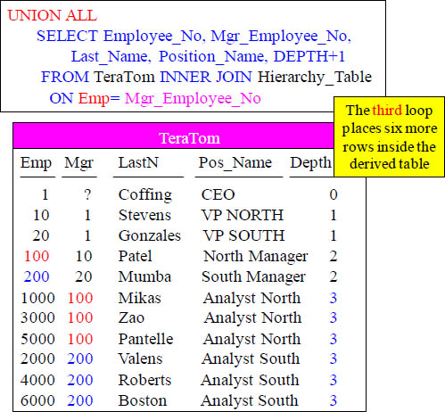
Six rows are added in the third loop.
WITH RECURSIVE Derived Table Ends the Looping

No rows were added in the fourth loop. This loop is done!
WITH RECURSIVE Derived Table Definition
Above is our WITH Recursive query and the highlighted part is now run so the final answer set can be delivered.
WITH RECURSIVE Derived Table Definition

The answer set is delivered.
Creating a Volatile Table

This statement creates a Volatile Table!
You Populate a Volatile Table with an INSERT/SELECT

Volatile tables are
Materialized with
An Insert/Select
statement
1) A USER Creates a Volatile Table and then 2) populates the Volatile Table with an INSERT/SELECT Statement. The space to materialize this table comes from the User’s Spool space. Now you can query this table all session long. When the session is logged off the table and the data are automatically deleted.
The Three Steps to Use a Volatile Table
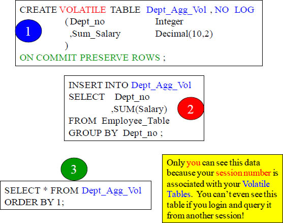
1) A USER Creates a Volatile Table and then 2) populates the Volatile Table with an INSERT/SELECT Statement, and then 3) Query it until you Logoff.
Why Would You Use the ON COMMIT DELETE ROWS?
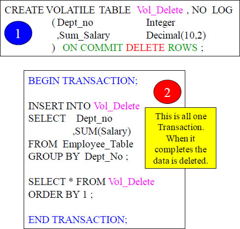
If you want to populate a Volatile Table and then only run one query then why not delete the data when you are done? That is what will happen in the above example. Now you are freeing up spool space that was used to keep the table materialized.
The HELP Volatile Table Command Shows your Volatiles
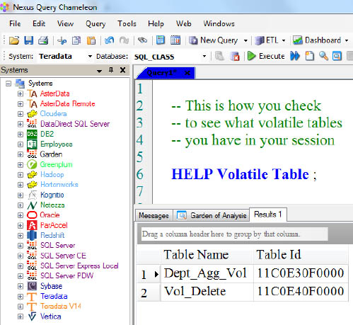
The HELP Volatile Table command above is exactly what you type in. This shows you all the Volatile tables you have materialized in your current session.
A Volatile Table with a Primary Index
CREATE Volatile TABLE Order_Vol, NO LOG
( OrderNo Integer NOT NULL
,CustNo Integer
,Order_Date Date
,Order_Total Decimal(10,2)
) PRIMARY INDEX (CustNo)
ON COMMIT PRESERVE ROWS ;
INSERT INTO Order_Vol
SELECT * FROM Order_Table
WHERE extract(Year from Order_Date) = 1999;
SELECT Customer_Name, O.*
FROM Order_Vol as O
INNER JOIN
SQL_Class.Customer_Table as C
ON C.Customer_Number = O.CustNo ;
It is a great idea to give your Volatile Table a Primary Index so you can control how it is distributed and the best way you want to query it. In the above example we knew we would be joining the Order_Vol directly to the Customer_Table with a join condition of CustNo=Customer_Number. We made sure that CustNo was the Primary Index of the Order_Vol table so the join could take place without any redistribution or duplication. The matching rows were already on the same AMPs.
The Joining of Two Tables Using a Volatile Table
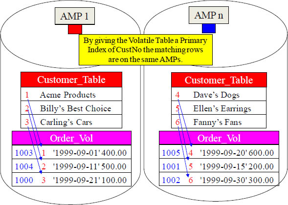
When Teradata does a join the matching rows need to be on the same AMP. We gave our Volatile Table a great Primary Index fully knowing we were going to populate it with 1999 orders and then join it to the Customer_Table on the join condition of CustNo. Now no data movement is required. Brilliant!
You Can Collect Statistics on Volatile Tables
You can Collect Statistics on Volatile Tables. This can help improve query performance. Consider collecting on:
All Non-Unique Primary Indexes (NUPI)
The Unique Primary Index of small tables
(less than 1,000 rows per AMP)
Columns that frequently appear in WHERE search conditions
Non-indexed columns used in joins
Partitioning column of a PPI Table
You don’t have to collect statistics on Volatile tables, but sometimes you will find if you are having performance problems that collecting statistics on a volatile table can greatly enhance performance. Above are some great guidelines for collecting statistics on volatile tables.
The New Teradata V14 Way to Collect Statistics
In previous versions Teradata required that you had to Collect Statistics for each column separately, thus always performing a full table scan each time. Those days are over!
| Old Way | New Teradata V14 Way |
|
COLLECT STATISTICS COLUMN (OrderNo, CustNo) ON Order_Vol ; COLLECT STATISTICS COLUMN (CustNo) ON Order_Vol; COLLECT STATISTICS ON Order_Vol Column (Order_Date) ; |
COLLECT STATISTICS COLUMN (OrderNo, CustNo) , COLUMN (CustNo) , COLUMN (Order_Date) ON Order_Vol; |
The new way to collect statistics in Teradata V14 is to do it all at the same time. This is a much better strategy. Only a single table scan is required, instead of 3 table scans using the old approach. This is an incredible improvement.
Some Great Examples of Creating a Volatile Table Quickly
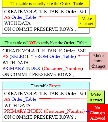
Above are two great examples to quickly CREATE a Volatile Table from another table. Our third example errors.
Creating Partitioned Primary Index (PPI) Volatile Tables
CREATE VOLATILE TABLE Order_Vol_PPI
AS ( SELECT * FROM Order_Table
WHERE Order_Date BETWEEN
DATE '2013-01-01' and '2013-06-30')
WITH DATA
PRIMARY INDEX (Order_Number)
PARTITION BY RANGE_N( ORDER_DATE
BETWEEN Date '2013-01-01' and Date '2013-06-30'
EACH INTERVAL '1' DAY)
ON COMMIT PRESERVE ROWS ;
Above you can see an example of quickly creating a Volatile Partitioned table directly from the actual Order_Table. We only inserted some of the data with our WHERE clause and we partitioned by day.
A Volatile Table That Only Populates Some of the Rows
Create a Volatile Table with orders from September
CREATE VOLATILE TABLE Order_Vol
AS (SELECT * FROM Order_Table
WHERE Extract(Month from Order_Date) = 9)
WITH DATA PRIMARY INDEX (Customer_Number)
ON COMMIT PRESERVE ROWS ;
Above is an example of creating a Volatile table that is not an exact copy. It is only populating the table with orders from the month of September.
A Volatile Table With No Data
This creates a table with no data
CREATE VOLATILE TABLE Order_Vol4
AS (SELECT * FROM Order_Table)
WITH NO DATA
PRIMARY INDEX(Customer_Number)
ON COMMIT PRESERVE ROWS ;
You must have either
WITH DATA
or
WITH NO DATA
INSERT INTO Order_Vol4
SELECT * FROM SQL_Class.Order_Table ;
Above is an example of creating a Volatile with no data. This must be further populated with an Insert/Select.
A Volatile Table With Some of the Columns
This creates a table with only three columns
CREATE VOLATILE TABLE Order_Vol5
AS (SELECT Customer_Number
,Order_Date, Order_Total
FROM Order_Table)
WITH DATA
ON COMMIT PRESERVE ROWS ;
Above is an example of creating a Volatile with three columns. The original table had four columns.
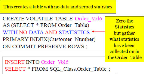
A Volatile Table With No Data and Zeroed Statistics
Collect Statistics ON Order_Vol6 ;
The same statistics
(columns/indexes)
from the Order_Table
are now recollected
for the Order_Vol6 table
Above is an example of creating a Volatile with no data and zeroed statistics. This must be further populated with an Insert/Select. Since the original Volatile table had no data, but statistics the statistics are all set to zero. When the table is populated with an Insert/Select it now has data. When the Collect Statistics command is run the same statistics that were collected on the Order_Table will be recollected on the Volatile table. That is the purpose of zeroed statistics.
A Multiset Volatile Table With Statistics Example

Above is an example of creating a Volatile table that is a Multiset table. A Multiset table allows duplicate rows, but a Set table deletes any rows that are duplicated in their entirety. It also brings over the statistics from the Order_Table.
Using a Volatile Table to Get Rid of Duplicate Rows
This Multiset table has duplicate rows and we want to get rid of them
CREATE VOLATILE SET TABLE Rid_Of_Dups
AS ( SELECT * FROM Sales_Table)
WITH DATA
ON COMMIT PRESERVE ROWS;
DELETE FROM Sales_Table All;
INSERT INTO Sales_Table
SELECT * from Rid_Of_Dups ;
If you have a Multiset table that accidentally gets unwanted duplicate rows you can use the technique above to get rid of them. We first create a SET Volatile table and when the data is copied the duplicate rows are eliminated. Then we can delete all the rows from the Multiset table and then reinsert the rows from the Volatile and all is good.
CREATING A Global Temporary Table
The Table Definition stays Permanently. When a user logs off the data inside the Global Temporary Table is deleted, but the definition stays around ready to be populated again.
CREATE Global Temporary TABLE Dept_Agg_GLO
( Dept_no Integer
,Sum_Salary Decimal(10,2)
)
ON COMMIT PRESERVE ROWS ;
ON COMMIT PRESERVE ROWS is NOT the default. You must us these Keywords if you want your data to stay in the Global Temporary Table after you populate it, otherwise after the load transaction the data is deleted. That is referred to as ON COMMIT DELETE ROWS.
Any user with Temp Space may materialize the
table. Each user who does gets their own copy.
This syntax creates a Global Temporary Table, which is stored in the Data Dictionary of Teradata. A Global Temporary Table survives a Teradata Restart.
Many Users Can Populate the Same Global Temporary Table

Above we see two users populating the Dept_Agg_GLO Global Temporary Table. Both users will get their own table. They have different data and neither can see the other’s table. Up to 2,000 users can populate a Global Temporary Table simultaneously. Each gets their own secure version of the data. When they logoff only the data is deleted.
Global Temporary Table with a Primary Index and Compress

INSERT INTO Order_Global
SELECT * FROM Order_Table
WHERE extract(Year from Order_Date) = 1999;

It is a great idea to give your Global Temporary Table a Primary Index so you can control how it is distributed and the best way you want to query it. In the above example we knew we would be joining the Order_Global directly to the Customer_Table with a join condition of CustNo = Customer_Number. We made sure that CustNo was the Primary Index of the Order_Vol table so the join could take place without any redistribution or duplication. The Compress key words will not use any space for null values.