Chapter 2 - Four Options for Aster Data Table Design
“Speak in a moment of anger and you’ll deliver the greatest speech you’ll ever regret.”
– Anonymous
There are Four Options to Aster Table Design
1. Straight up Distribute by Hash:
All of your fact tables will use the Distribute by Hash design of simply having a single column serving as the Distribution Key. These tables will distribute the rows of the table among the vworkers with a consistent and straightforward Hash Formula.
2. Straight up Distribute by Replication:
Most of your dimension tables will use the Distribute by Replication design which makes a complete copy of all rows in the table and distributes the entire copy across all vworkers. Each vworker has an exact copy of the entire table.
3. Partition the table with Logical Partitioning:
Aster allows a table to be created with a horizontal partition. The Distribution Key distributes the rows among the vworkers just like a traditional table, but each vworker sorts the data on the partition. All vworkers will be involved in retrieving an answer set, but each vworker only reads the data held in particular partitions, thus no longer performing a Full Table Scan.
4. Columnar Design:
Aster allows for tables to be created in a Columnar design. The rows are distributed in their entirety among the vworkers, but the rows break each column up into their own blocks. This is considered vertical partitioning and a great design for queries only needing a few columns.
Straight up Distribute by Hash
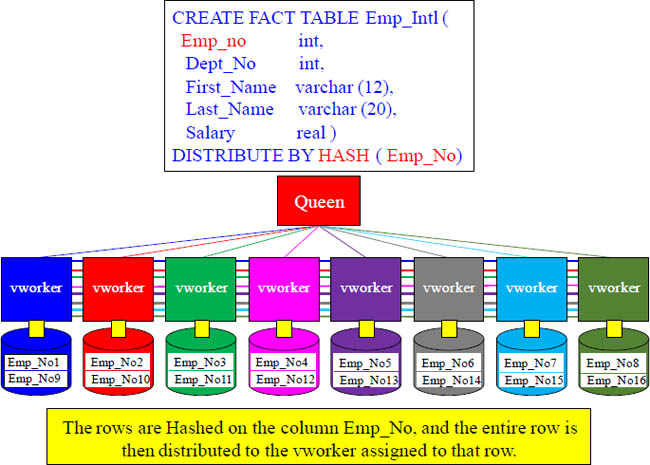
Aster Hashes the Distribution Key with a single formula and then distributes the rows among the vworkers.
Straight up Distribute by Hash - Problems
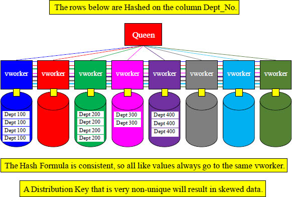
Aster Hashes the Distribution Key with a single formula and then distributes the rows among the vworkers. All like values go to the same vworker. Be careful what Distribution Key you choose.
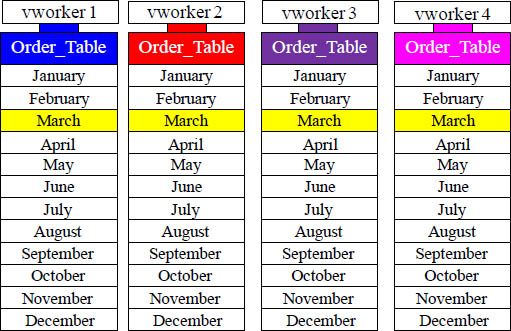
Straight up Distribute by Replication
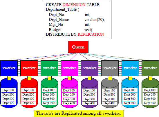
A Replicated table means that each vworker holds the entire table. Each row is duplicated on every vworker.
Partition the Table with Logical Partitioning
CREATE FACT TABLE orders_partitioned (
order_id int NOT NULL
,customer_id int
,daily_sales int
,order_date timestamp )
DISTRIBUTE BY HASH(order_id)
PARTITION BY RANGE(order_date)
( PARTITION jan_2014( END '2014-02-01' ),
PARTITION feb_2014( END '2014-03-01' ),
PARTITION mar_2014( END '2014-04-01' ),
PARTITION apr_2014( END '2014-05-01' ),
PARTITION may_2014( END '2014-06-01' ),
PARTITION Jun_2014( END '2014-07-01' ),
PARTITION jul_2014( END '2014-08-01' ),
PARTITION aug_2014( END '2014-09-01' ),
PARTITION sep_2014( END '2014-10-01' ),
PARTITION oct_2014( END '2014-11-01' ),
PARTITION nov_2014( END '2014-12-01' ),
PARTITION dec_2014( END '2015-01-01' ) ) ;
The table is distributed by order_id, but each vworker places each partition in a separate data block. Look at the next page to see a visual of the AMPs and their sorting of millions of rows.
This Partitioned Table Sorts Rows by Month of Order_Date
Each vworker above sorts their rows by Month (of Order_Date), so if a user queries and only wants to see the orders placed in March, then each vworker just transfers the blocks with March orders. This is an all vworker retrieve, but each vworker only has to retrieve from a single partition, which is the March Partition. The entire reason for logical partitioning is to eliminate a full table scan especially on range queries.
An All vworkers Retrieve By Way of a Single Partition
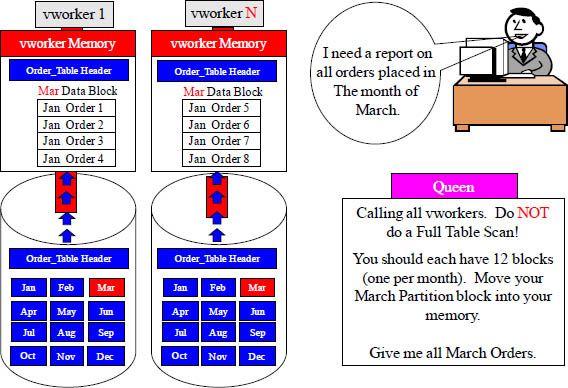
All vworkers are used to satisfy the query, but each vworker only reads one partition.
You can Partition a Table by Range or by List
CREATE FACT TABLE Sales_By_Region
(
sales_id int,
region_id char(5),
state varchar,
date_time timestamp,
revenue int
)
DISTRIBUTE BY HASH(sales_id)
PARTITION BY LIST(region_id)
(
PARTITION region1( VALUES('North') ),
PARTITION region2( VALUES('South') ),
PARTITION region3( VALUES('East') ),
PARTITION region4( VALUES('West'))
);
A Fact or a Dimension table can be partitioned by Range or List or a combination of both. Above, we have created a Fact table and partitioned by list. We have four partitions. Notice that the rows are hashed to their vworker on sales_id, but once they arrive at the vworker they are sorted (partitioned) by the region_name. If users use the sales_id in the WHERE clause, then only the vworker holding that row will be contacted. If region_name is used in the WHERE clause, then all vworkers will be contacted, but each vworker will only look in the partition that holds that particular region_name.
A Partitioned By List Example with Three Tactical Queries
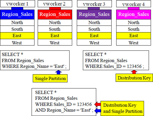
Above are queries that are tuned for speed. Which one is the fastest? The bottom example!
Aster Data Multi-Level Partitioning
CREATE FACT TABLE Orders_Partitioned
( order_id int NOT NULL
,customer_id int
,daily_sales int
,order_date timestamp
,region_name Char(5)
) DISTRIBUTE BY HASH(order_id)
PARTITION BY RANGE(order_date)
( PARTITION qtr1( END '2014-03-31' ),
PARTITION qtr2( END '2014-06-30' ),
PARTITION qtr3( END '2014-09-30' ),
PARTITION qtr4( END '2014-12-31'
PARTITION BY LIST(region_name)
(
PARTITION region1( VALUES('North') ),
PARTITION region2( VALUES('South') ),
PARTITION region3( VALUES('East') ),
PARTITION region4( VALUES('West') )
)));
The Orders_Partitioned table above has multi-level partitioning (by quarter and then by region name).
Aster Allows for Multi-Level Partitioning
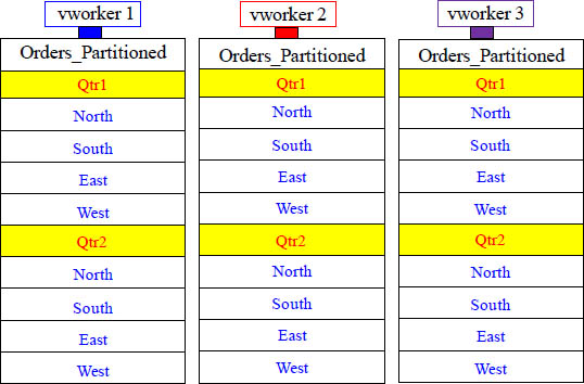
The table was hashed by Order_ID. Then, it was partitioned by Quarter (Jan, Feb, Mar are the 1st quarter), and finally, it was partitioned by Region_Name (North, South, East or West).
SQL Commands for Logical Partitioning as One Table
• INSERT
• CREATE INDEX
• SELECT
• UPDATE
• DELETE
• MERGE
• COPY
• TRUNCATE
• VACUUM
• ANALYZE
• CLUSTER
• REINDEX
• ALTER
• GRANT, and
• REVOKE
The SQL commands above operate on the logical partitioned table hierarchy as if it were one table. Issue the command against the top level table, and it will automatically cascade to the correct child partition.
What Partitions are on my Table?
SELECT ucp.*
FROM nc_user_child_partitions AS ucp
INNER JOIN
nc_user_tables AS ust
ON ust.tableid = ucp.tableid
WHERE ust.tablename = 'orders_partitioned' ;
The query above uses Aster Data system tables to show a table with multi-level partitioning.
Information on the partitions is available by accessing system tables. If the table has a multi-level partitioning, the above query will show all levels.
What does a Columnar Table look like?
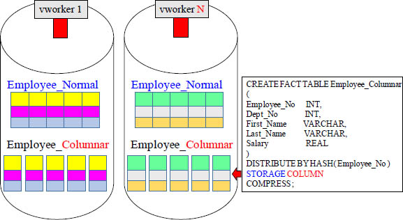
Aster Database supports Columnar tables, and this option is available for distributed, replicated, and logically partitioned tables including temporary and persistent tables. If the majority of your queries access a low percentage of the columns of a given table, then it may be a good candidate for columnar. The two tables above contain the same Employee data, but the bottom example is a Columnar table. Employee_Normal has 3 rows on each AMP with 5 columns. Employee_Columnar is split into 5 different blocks.
A Comparison of Data for Normal Vs. Columnar
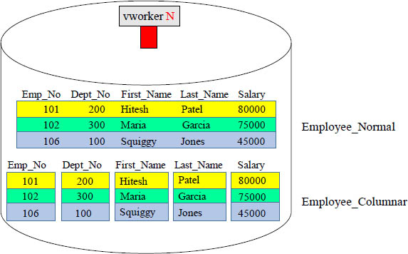
The normal table on top is one block containing three rows and five columns. The columnar table below has five blocks each containing one column of three rows. Columnar tables are better when users query just a few columns and not all columns.
A Columnar Table is best for Queries with Few Columns
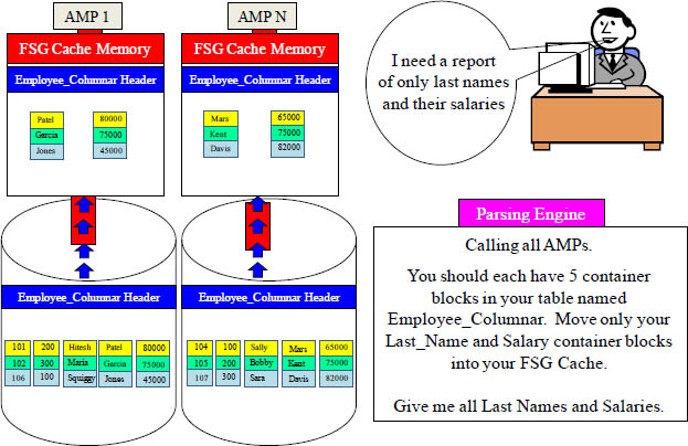
All rows come back but only two columns. We moved less than half the block volume.
Quiz – How Many Blocks Move to vworker Memory?
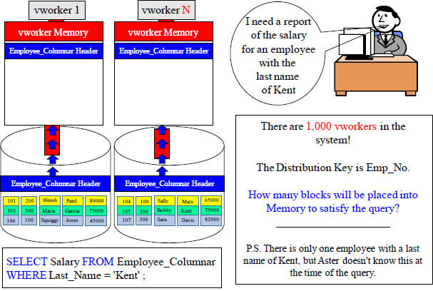
Your mission is to think! Remember that the Queen does the least work always.
Answer – How Many Containers Move to vworker Memory?
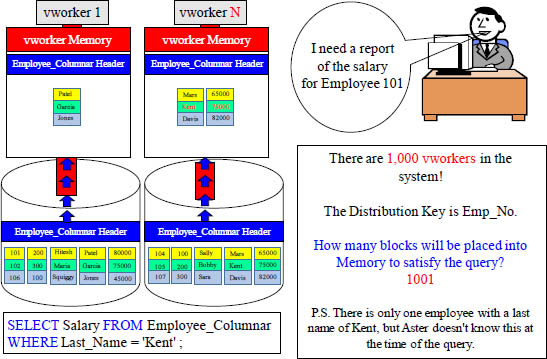
All 1,000 vworkers place only their Last_Name block in memory, and then when a vworker finds an Employee named Kent, they move their Salary container into their memory. Did you think 2000?
When to use a Columnar Table
The data rarely changes (no UPDATE, no DELETE, and few INSERT statements or load/ COPY operations).
A large percentage of the queries use aggregate functions.
A large percentage of the queries use ORDER BY or GROUP BY on a specific column (which is of course the column on which we would want to create the index that will be used to CLUSTER).
If a table has many columns that include wide columns, such as varchar, the queries generally involve the non-wide columns.
Above is a description of tables that generally might be candidates for Columnar.