
Chapter 12 Agitated atoms: Materials and heat
- 12.1 Introduction and synopsis 244
- 12.2 Thermal properties: definition and measurement 244
- 12.3 The big picture: thermal property charts 248
- 12.4 Drilling down: the physics of thermal properties 251
- 12.5 Manipulating thermal properties 255
- 12.6 Design to exploit thermal properties 257
- 12.7 Summary and conclusions 266
- 12.8 Further reading 267
- 12.9 Exercises 267
- 12.10 Exploring design with CES 269
- 12.11 Exploring the science with CES Elements 270
12.1 Introduction and synopsis
Thermal properties quantify the response of materials to heat. Heat, until about 1800, was thought to be a physical substance called ‘caloric’ that somehow seeped into things when they were exposed to flame. It took the American Benjamin Thompson1, backed up by none other than the formidable Carnot2, to suggest what we now know to be true: that heat is atoms or molecules in motion. In gases, they are flying between occasional collisions with each other. In solids, by contrast, they vibrate about their mean positions; the higher the temperature, the greater the amplitude of vibrations. From this perception emerges all of our understanding of thermal properties of solids: their heat capacity, expansion coefficient, conductivity, even melting.
Heat affects mechanical and physical properties too. As temperature rises, materials expand, the elastic modulus decreases, the strength falls and the material starts to creep, deforming slowly with time at a rate that increases as the melting point is approached until, on melting, the solid loses all stiffness and strength. This we leave for Chapter 13.
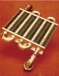
Thermal design, the ultimate topic of this chapter, is design to cope properly with the effects of heat or, where possible, to exploit them. The chapter opening page shows an example: a copper heat exchanger, designed to transfer heat efficiently between two circulating fluids.
12.2 Thermal properties: definition and measurement
Two temperatures, the melting temperature, Tm, and the glass temperature, Tg (units for both: kelvin3, K, or centigrade, °C) are fundamental points of reference because they relate directly to the strength of the bonds in the solid. Crystalline solids have a sharp melting point, Tm. Non-crystalline solids do not; the glass temperature Tg characterises the transition from true solid to very viscous liquid. It is helpful, in engineering design, to define two further temperatures: the maximum and minimum service temperatures, Tmax and Tmin (units for both: K or °C). The first tells us the highest temperature at which the material can be used continuously without oxidation, chemical change or excessive distortion becoming a problem. The second is the temperature below which the material becomes brittle or otherwise unsafe to use.
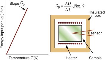
It costs energy to heat a material up. The energy to heat 1 kg of a material by 1 K is called the heat capacity or specific heat, and since the measurement is usually made at constant pressure (atmospheric pressure) it is given the symbol Cp. Heat is measured in Joules4, symbol J, so the units of specific heat are J/kg · K. When dealing with gases, it is more usual to measure the heat capacity at constant volume (symbol Cv), and for gases this differs from Cp. For solids the difference is so slight that it can be ignored, and we shall do so here. Cp is measured by the technique of calorimetry, which is also the standard way of measuring the glass temperature Tg. Figure 12.1 shows how, in principle, this is done. A measured quantity of energy (here, electrical energy) is pumped into a sample of material of known mass. The temperature rise is measured, allowing the energy/kg.K to be calculated. Real calorimeters are more elaborate than this, but the principle is the same.
Most materials expand when they are heated (Figure 12.2). The thermal strain per degree of temperature change is measured by the linear thermal expansion coefficient, α. It is defined by
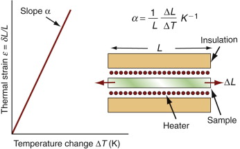
Figure 12.2 Measuring the thermal expansion coefficient, α. Its units are 1/K or, more usually, 10–6/K (microstrain/K).

where L is a linear dimension of the body. If the material is anisotropic it expands differently in different directions, and two or more coefficients are required. Since strain is dimensionless, the units of α are K–1 or, more conveniently, ‘microstrain/K’, that is, 10–6 K–1.
Example 12.1
The volume of water in the earth’s oceans is V = 1.37 × 10⁹ km3. The oceans cover an area A = 3.61 × 10⁸ km2 (71% of the earth’s surface). Thus the average depth is 3795 m. The average surface temperature is 17 °C, but the deeper water is colder—we take the average to be 10 °C. The volumetric coefficient of thermal expansion of water at 10 °C, αv = 8.8 × 10⁻⁵ K−1. If the earth’s oceans warmed by 2 °C, by how much would sea level rise?
Answer. The volume change caused by the temperature rise is ΔV = αv.V.ΔT = 2.4× 10⁸ m3. Dividing this by the surface area of the oceans gives a rise of 0.66 m.
Example 12.2
A steel rail of square cross-section 25 mm × 25 mm is rigidly clamped at two points a distance L = 2 m apart. If the rail is stress-free at 20 °C, at what temperature will thermal expansion cause it to buckle elastically? (The thermal expansion coefficient of steel is α = 12 × 10−6/K.)
Answer. The elastic buckling load of a column clamped in this way is given by equation (5.9) and Figure 5.5:

Here E is Young’s modulus and ![]() is the second moment of area of the rail. When the clamped rail is heated by ΔT it expands, causing a stress σ = EαΔT to appear in it. The clamps there exert an axial load F = σA = EAαΔT on the rail, where A = 6.25 × 10⁻⁴ m2 is the area of its cross-section. Equating this to Fcrit and solving for ΔT gives
is the second moment of area of the rail. When the clamped rail is heated by ΔT it expands, causing a stress σ = EαΔT to appear in it. The clamps there exert an axial load F = σA = EAαΔT on the rail, where A = 6.25 × 10⁻⁴ m2 is the area of its cross-section. Equating this to Fcrit and solving for ΔT gives
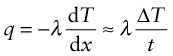
Power is measured in Watts5; 1 Watt (W) is 1 Joule/second. The rate at which heat is conducted through a solid at steady-state (meaning that the temperature profile does not change with time) is measured by the thermal conductivity, λ (units: W/m.K). Figure 12.3 shows how it is measured: by recording the heat flux q (W/m2) flowing through the material from a surface at higher temperature T1 to a lower one at T2 separated by a distance x. The conductivity is calculated from Fourier’s6 law:
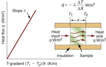
where q is the heat flux per unit area (units: W/m2).
Thermal conductivity, as we have said, governs the flow of heat through a material at steady-state. The property governing transient heat flow (when temperature varies with time) is the thermal diffusivity, a (units: m2/s). The two are related by

where ρ is the density and Cp is, as before, the heat capacity. The thermal diffusivity can be measured directly by measuring the time it takes for a temperature pulse to traverse a specimen of known thickness when a heat source is applied briefly to the one side; or it can be calculated from λ (and ρCp) via equation (12.3).
12.3 The big picture: thermal property charts
Three charts give an overview of thermal properties and their relationship to strength.
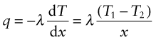
Thermal expansion, α, and thermal conductivity, λ
Figure 12.4 maps thermal expansion, α, and thermal conductivity, λ. Metals and technical ceramics lie toward the lower right: they have high conductivities and modest expansion coefficients. Polymers and elastomers lie at the upper left: their conductivities are 100 times less and their expansion coefficients 10 times greater than those of metals. The chart shows contours of λ/α, a quantity important in designing against thermal distortion—a subject we return to in Section 12.6. An extra material, Invar (a nickel alloy), has been added to the chart because of its uniquely low expansion coefficient at and near room temperature, a consequence of a trade-off between normal expansion and a contraction associated with a magnetic transformation.
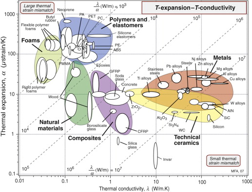
Figure 12.4 The linear expansion coefficient, α, plotted against the thermal conductivity, λ. The contours show the thermal distortion parameter λ/α.
Thermal conductivity, λ, and thermal diffusivity, a
Figure 12.5 shows the room temperature values of thermal conductivity, λ, and thermal diffusivity, a, with contours of volumetric heat capacity ρCp, equal to the ratio of the two, λ/α (from equation (12.3)). The data span almost five decades in λ and a. Solid materials are strung out along the line
Figure 12.5 The thermal conductivity, λ, plotted against the thermal diffusivity, a = λ/ρCp. The contours show the specific heat per unit volume ρCp.
meaning that the heat capacity per unit volume, ρCp, is almost constant for all solids, something to remember for later. As a general rule, then,
(λ in W/m.K and a in m2/s). Some materials deviate from this rule: they have lower-than-average volumetric heat capacity. The largest deviations are shown by porous solids: foams, low-density firebrick, woods and the like. Because of their low density they contain fewer atoms per unit volume and, averaged over the volume of the structure, ρCp is low. The result is that, although foams have low conductivities (and are widely used for insulation because of this), their thermal diffusivities are not necessarily low. This means that they don’t transmit much heat, but they do change temperature quickly.
Example 12.4
A locally available building material in a third-world country has a density that you find by weighing a cube of known dimensions to be ρ = 2300 kg/m3. To judge the thermal behaviour of the shelter you are proposing to build you wish to know its heat capacity Cp. What would you estimate it to be?
Answer. The chart of Figure 12.5 shows that, for solids, the quantity ρCp ≈ 3 × 10⁶ J/m3.K so the heat capacity of the material is Cp ≈ 1300 J/kg.K.
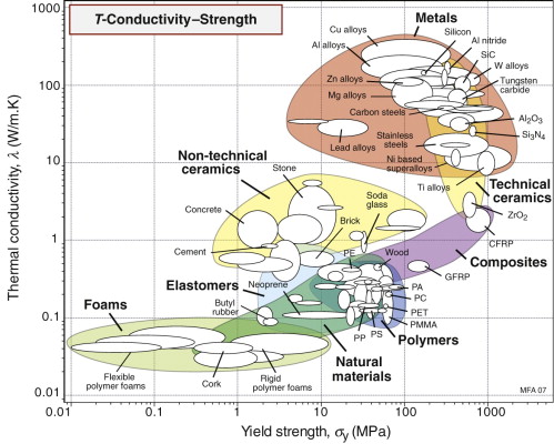
Thermal conductivity λ and yield strength σy
The final chart, Figure 12.6, shows thermal conductivity, λ and strength, σy. Metals, particularly the alloys of copper, aluminum and nickel, are both strong and good conductors, a combination of properties we seek for applications such as heat exchangers—one we return to in Section 12.6.
12.4 Drilling down: the physics of thermal properties
Heat capacity
We owe our understanding of heat capacity to Albert Einstein7 and Peter Debye8. Heat, as already mentioned, is atoms in motion. Atoms in solids vibrate about their mean positions with an amplitude that increases with temperature. Atoms in solids can’t vibrate independently of each other because they are coupled by their inter-atomic bonds; the vibrations are like standing elastic waves. Figure 12.7 shows how, along any row of atoms, there is the possibility of one longitudinal mode and two transverse modes, one in the plane of the page and one normal to it. Some of these have short wavelengths and high energy, others long wavelengths and lower energy (Figure 12.8). The shortest possible wavelength, λ1, is just twice the atomic spacing; the other vibrations have wavelengths that are longer. In a solid with N atoms there are N discrete wavelengths, and each has a longitudinal mode and two transverse modes, 3N modes in all. Their amplitudes are such that, on average, each has energy kBT, where kB is Boltzmann’s constant9, 1.38 × 10⁻²³ J/K. If the volume occupied by an atom is Ω, then the number of atoms per unit volume is N = 1/Ω and the total thermal energy per unit volume in the material is 3kBT/Ω. The heat capacity per unit volume, ρCp, is the change in this energy per Kelvin change in temperature, giving:
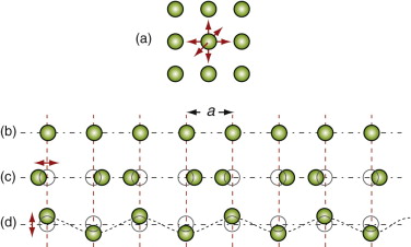
Figure 12.7 (a) An atom vibrating in the ‘cage’ of atoms that surround it with three degrees of freedom. (b) A row of atoms at rest. (c) A longitudinal wave. (d) One of two transverse waves (in the other the atoms oscillate normal to the page).
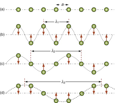
Figure 12.8 Thermal energy involves atom vibrations. There is one longitudinal mode of vibration and two transverse modes, one of which is shown here. The shortest meaningful wavelength, λ1 = 2a, is shown in (b).
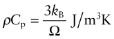
Atomic volumes do not vary much; all lie within a factor of 3 of the value 2 × 10–29/m3, giving a volumetric heat capacity
The chart of Figure 12.5 showed that this is indeed the case.
Thermal expansion
If a solid expands when heated (and almost all do) it must be because the atoms are moving farther apart. Figure 12.9 shows how this happens. It looks very like an earlier one, Figure 4.22, but there is a subtle difference: the force–spacing curve, a straight line in the earlier figure, is not in fact quite straight; the bonds become stiffer when the atoms are pushed together and less stiff when they are pulled apart. Atoms vibrating in the way described earlier oscillate about a mean spacing that increases with the amplitude of oscillation, and thus with increasing temperatures. So thermal expansion is a nonlinear effect; if the bonds between atoms were linear springs, there would be no expansion.
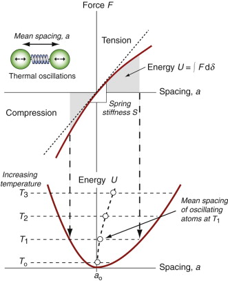
Figure 12.9 Thermal expansion results from the oscillation of atoms in an unsymmetrical energy well.
The stiffer the springs, the steeper is the force–displacement curve and the narrower is the energy well in which the atom sits, giving less scope for expansion. Thus, materials with high modulus (stiff springs) have low expansion coefficient, those with low modulus (soft springs) have high expansion—indeed, to a good approximation

(E in GPa, α in K–1). It is an empirical fact that all crystalline solids expand by about the same amount on heating from absolute zero to their melting point: it is about 2%. The expansion coefficient is the expansion per degree Kelvin, meaning that

For example, tungsten, with a melting point of around 3330 °C (3600 K) has α = 5 × 10⁻⁶/°C, while lead, with a melting point of about 330 °C (600 K, six times lower) expands six times more (α = 30 × 10–6/°C). Equation (12.9) (with Tm in Kelvin, of course) is a remarkably good approximation for the expansion coefficient. Note in passing that equations (12.8) and (12.9) indicate that E is expected to scale with Tm—try exploring how well these approximations hold using the CES Elements database.
Thermal conductivity
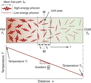
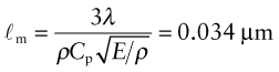
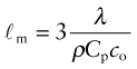
Heat is transmitted through solids in three ways: by thermal vibrations; by the movement of free electrons in metals; and, if they are transparent, by radiation. Transmission by thermal vibrations involves the propagation of elastic waves. When a solid is heated the heat enters as elastic wave packets or phonons. The phonons travel through the material and, like any elastic wave, they move with the speed of sound, ![]() . If this is so, why does heat not diffuse at the same speed? It is because phonons travel only a short distance before they are scattered by the slightest irregularity in the lattice of atoms through which they move, even by other phonons. On average they travel a distance called the mean free path, ℓm, before bouncing off something, and this path is short: typically less than 0.01 µm (10–8 m).
. If this is so, why does heat not diffuse at the same speed? It is because phonons travel only a short distance before they are scattered by the slightest irregularity in the lattice of atoms through which they move, even by other phonons. On average they travel a distance called the mean free path, ℓm, before bouncing off something, and this path is short: typically less than 0.01 µm (10–8 m).
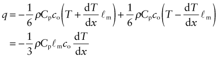
We calculate the conductivity by using a net flux model, much as you would calculate the rate at which cars accumulate in a car park by counting the rate at which they enter and subtracting the rate at which they leave. Phonon conduction can be understood in a similar way, as suggested by Figure 12.10. Here a rod with unit cross-section carries a uniform temperature gradient dT/dx between its ends. Phonons within it have three degrees of freedom of motion (they can travel in the ±x, the ±y and the ±z directions). Focus on the midplane M–M. On average, one-sixth of the phonons are moving in the +x direction; those within a distance ℓm of the plane will cross it from left to right before they are scattered, carrying with them an energy ρCp(T + ΔT) where T is the temperature at the plane M–M and ΔT = (dT/dx)ℓm. Another one-sixth of the phonons move in the –x direction and cross M–M from right to left, carrying an energy ρCp(T – ΔT). Thus, the energy flux qJ/m2.s across unit area of M–M per second is
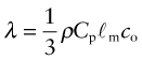
Comparing this with the definition of thermal conductivity (equation (12.2)), we find the conductivity to be
Sound waves, which, like phonons, are elastic waves, travel through the same bar without much scattering. Why do phonons scatter so readily? It’s because waves are scattered most by obstacles with a size comparable with their wavelengths—that is how diffraction gratings work. Audible sound waves have wavelengths of metres, not microns; they are scattered by buildings (which is why you can’t always tell where a police siren is coming from) but not by the atom-scale obstacles that scatter phonons, with wavelengths starting at two atomic spacings (Figure 12.8).
Elastic waves contribute little to the conductivity of pure metals such as copper or aluminum because the heat is carried more rapidly by the free electrons. Equation (12.10) still applies but now Cp, co and ℓm become the thermal capacity, the velocity and the mean free path of the electrons. Free electrons also conduct electricity, with the result that metals with high electrical conductivity also have high thermal conductivity (the Wiedemann–Franz law), as will be illustrated in Chapter 14.
12.5 Manipulating thermal properties
Thermal expansion
Expansion, as already mentioned, can generate thermal stress and cause distortion, undesirable in precise mechanisms and instruments. The expansion coefficient α, like modulus or melting point, depends on the stiffness and strength of atomic bonds. There’s not much you can do about these, so the expansion coefficient, normally, is beyond our control. Some few materials have exceptionally low expansion—borosilicate glass (Pyrex), silica and carbon fibres, for example—but they are hard to use in engineering structures. There is one exception: the family of alloys called Invars with very low expansion. They achieve this by the trick of canceling the thermal expansion (which is, in fact, happening) with a contraction caused by the gradual loss of magnetism as the material is heated.
Thermal conductivity and heat capacity
Equation (12.10) describes thermal conductivity. Which of the terms it contains can be manipulated and which cannot? The volumetric heat capacity ρCp, as we have seen, is almost the same for all solid materials. The sound velocity ![]() depends on two properties that are not easily changed. That leaves the mean free path, ℓm, of the phonons or, in metals, of the electrons. Introducing scattering centers such as impurity atoms or finely dispersed particles achieves this. Thus, the conductivity of pure iron is 80 W/m.K, while that of stainless steel—iron with up to 30% of nickel and chromium—is only 18 W/m.K. Certain materials can exist in a glassy state, and here the disordered nature of the glass makes every molecule a scattering center and the mean free path is reduced to a couple of atom spacings; the conductivity is correspondingly low.
depends on two properties that are not easily changed. That leaves the mean free path, ℓm, of the phonons or, in metals, of the electrons. Introducing scattering centers such as impurity atoms or finely dispersed particles achieves this. Thus, the conductivity of pure iron is 80 W/m.K, while that of stainless steel—iron with up to 30% of nickel and chromium—is only 18 W/m.K. Certain materials can exist in a glassy state, and here the disordered nature of the glass makes every molecule a scattering center and the mean free path is reduced to a couple of atom spacings; the conductivity is correspondingly low.
Chapter 6 showed how strength is increased by defects such as solute atoms, precipitates and work hardening. Some of these reduce the thermal conductivity. Figure 12.11 shows a range of aluminum alloys hardened by each of the three main mechanisms: solid solution, work hardening and precipitation hardening. Work hardening strengthens significantly without changing the conductivity much, while solid solution and precipitation hardening introduce more scattering centres, giving a drop in conductivity.
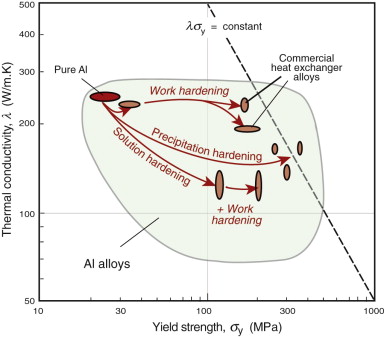
Figure 12.11 Thermal conductivity and strength for aluminum alloys. Good materials for heat exchangers have high values of λσy, indicated by the dashed line.
We are not, of course, restricted to fully dense solids, making density ρ a possible variable after all. In fact, the best thermal insulators are porous materials—low-density foams, insulating fabric, cork, insulating wool etc.—that take advantage of the low conductivity of still air trapped in the pores (λ for air is 0.02 W/m.K).
12.6 Design to exploit thermal properties
All materials have a thermal expansion coefficient α, a specific heat Cp and a thermal conductivity λ. Material property charts are particularly helpful in choosing materials for applications that use these. Certain thermal properties, however, are shown only by a few special materials: shape-memory behavior is an example. There is no point in making charts for these because so few materials have them, but they are still of engineering interest. Examples that use them are described nearer the end of the section.
Managing thermal stress
Most structures, small or large, are made of two or more materials that are clamped, welded or otherwise bonded together. This causes problems when temperatures change. Railway track will bend and buckle in exceptionally hot weather (steel, high α, clamped to mother earth with a much lower α). Overhead transmission lines sag for the same reason—a problem for high-speed electric trains. Bearings seize, doors jam. Thermal distortion is a particular problem in equipment designed for precise measurement or registration like that used to make masks for high-performance computer chips, causing loss of accuracy when temperatures change.
All of these derive from differential thermal expansion, which, if constrained (clamped in a way that stops it happening) generates thermal stress. As an example, many technologies involve coating materials with a thin surface layer of a different material to impart wear resistance, or resistance to corrosion or oxidation. The deposition process often operates at a high temperature. On cooling, the substrate and the surface layer contract by different amounts because their expansion coefficients differ and this puts the layer under stress. This residual stress is calculated as follows.
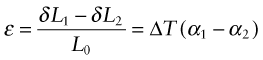
Think of a thin film bonded onto a component that is much thicker than the film, as in Figure 12.12(a). First imagine that the layer is detached, as in Figure 12.12(b). A temperature drop of ΔT causes the layer to change in length by δL1 = α1L0ΔT. Meanwhile, the substrate to which it was previously bonded contracts by δL2 = α2L0ΔT. If α1 > α2 the surface layer shrinks more than the substrate. If we want to stick the film back on the much-more-massive substrate, covering the same surface as before, we must stretch it by the strain
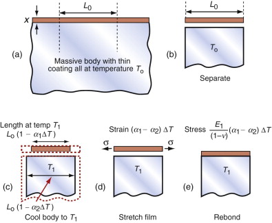
Figure 12.12 Thermal stresses in thin films arise on cooling or heating when their expansion coefficients differ. Here that of the film is α1 and that of the substrate, a massive body, is α2.
This requires a stress in the film of
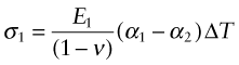
where the Poisson’s ratio term enters due to the biaxial stress state in the film. The stress can be large enough to crack the surface film. The pattern of cracks seen on glazed tiles arises in this way.
So if you join dissimilar materials you must expect thermal stress when they are heated or cooled. The way to avoid it is to avoid material combinations with very different expansion coefficients. The α–λ chart of Figure 12.4 has expansion α as one of its axes: benign choices are those that lie close together on this axis, dangerous ones are those that lie far apart.
But avoiding materials with α mismatch is not always possible. Think of joining glass to metal—Pyrex to stainless steel, say—a common combination in high vacuum equipment. Their expansion coefficients can be read from the α–λ chart of Figure 12.4: for Pyrex (borosilicate glass), α = 4 × 10⁻⁶/K; for stainless steel, α = 20 × 10–6/K: a big mismatch. Vacuum equipment has to be ‘baked out’ to desorb gases and moisture, requiring that it be heated to about 150 °C, enough for the mismatch to crack the Pyrex. The answer is to grade the joint with one or more materials with expansion that lies between the two: first join the Pyrex to a glass of slightly higher expansion and the stainless to a metal of lower expansion—the chart suggests soda glass for the first and a nickel alloy for the second—and then diffusion-bond these to each other, as in Figure 12.13. The graded joint spreads the mismatch, lowering the stress and the risk of damage.
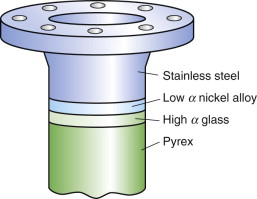
Figure 12.13 A graded joint. The high expansion stainless steel is bonded to a nickel alloy of lower expansion, the low expansion Pyrex (a borosilicate glass) is bonded to a glass with higher expansion, and the set is assembled to give a stepwise graded expansion joint.
There is an alternative, although it is not always practical. It is to put a compliant layer—rubber, for instance—in the joint; it is the way windows are mounted in cars. The difference in expansion is taken up by distortion in the rubber, transmitting very little of the mismatch to the glass or surrounding steel.
Thermal sensing and actuation
Thermal expansion can be used to sense (to measure temperature) and to actuate (to open or close valves or electrical circuits, for instance). The direct thermal displacement δ = αLoΔT is small; it would help to have a way to magnify it. Figure 12.14 shows one way to do this. Two materials, deliberately chosen to have different expansion coefficients α1 and α2, are bonded together in the form of a bi-material strip, of thickness 2t, as in Figure 12.14(a). When the temperature changes by ΔT = (T1 – To), one expands more than the other, causing the strip to bend. The mid-thickness planes of each strip (dotted in Figure 12.14(b)) differ in length by Lo(α2 – α1)ΔT. Simple geometry then shows that
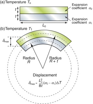
Figure 12.14 The thermal response of a bi-material strip when the expansion coefficients of the two materials differ. The configuration magnifies the thermal strain.
from which
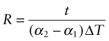
The resulting upward displacement of the centre of the bi-material strip (assumed to be thin) is
A large aspect ratio Lo/t produces a large displacement, and one that is linear in temperature.
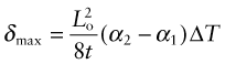
Thermal gradients
There is a subtler effect of expansion that causes problems even in a single material. Suppose a chunk of material is suddenly cooled by ΔT (by dropping it hot into a bath of cold water, for example) or suddenly heated by ΔT (by dropping it cold into boiling water). The surface, almost immediately, is forced to the temperature of the bath, as in Figure 12.15. It contracts (if cooled) or expands (if heated) by δL such that δL/Lo = αΔT. The inside of the material has not expanded yet—there has not been time for the heat to diffuse into it. That means there is a temperature gradient, and even though the material has just one expansion coefficient, there are different strains in different places. Since the surface is stuck to the interior, it is constrained, so thermal stresses appear in it just as they did in the thin film of Figure 12.12. In brittle materials, these stresses can cause fracture. The ability of a material to resist this, its thermal shock resistance, ΔTs (units: K or °C), is the maximum sudden change of temperature to which such a material can be subjected without damage.
Even if the stresses do not cause failure, temperature gradients lead to distortion. Which properties minimise this? Figure 12.15 shows the temperature profile in the quenched body at successive times τ1, τ2 … τ5. A cooling or heating front propagates inward from the surface by the process of heat diffusion discussed earlier—and while it is happening there is a temperature gradient and consequent thermal stress. If the material remains elastic, then the stresses fade away when the temperature is finally uniform—though the component may by then have cracked. If the material partially yields, the stresses never go away, even when the temperature profile has smoothed out, because the surface has yielded but the center has not. This residual stress is a major problem in metal processing, particularly welding, causing distortion and failure in service.
The important new variable here is time—it is this that distinguishes the contours in Figure 12.15. The material property that determines this time is the thermal diffusivity a that we encountered earlier:

with units of m2/s. The bigger the conductivity, λ, the faster the diffusivity, a, but why is ρCp on the bottom? If this quantity, the heat capacity per unit volume, is large, a lot of heat has to diffuse in or out of unit volume to change the temperature much. The more that has to diffuse, the longer it takes to do so, so that the diffusivity a is reduced. If you solve transient heat flow problems (of which this is an example), a general result emerges: it is that the characteristic distance x (in meters) that heat diffuses in a time τ (in seconds) is
This is a particularly useful little formula, and although approximate (because the constant of proportionality, here ![]() , actually depends somewhat on the geometry of the body into which the heat is diffusing), it is perfectly adequate for first estimates of heating and cooling times.
, actually depends somewhat on the geometry of the body into which the heat is diffusing), it is perfectly adequate for first estimates of heating and cooling times.
Example 12.6
A flat heat shield is designed to protect against sudden temperature surges. Its maximum allowable thickness is 10 mm. What value of thermal diffusivity is needed to ensure that, when heat is applied to one of its surfaces, the other does not start to change significantly in temperature for 5 minutes? Use the chart of Figure 12.5 to identify material that you might use for the heat shield.
Answer. The distance x moved by a thermal front in time t in a material of thermal diffusivity a is ![]() . Inserting the values of x (in m) and t (in seconds) gives a < 1.67 × 10⁻⁷ m2/s. According to Figure 12.5 almost all polymers have a thermal diffusivity that meets this constraint, but few materials of other classes meet it.
. Inserting the values of x (in m) and t (in seconds) gives a < 1.67 × 10⁻⁷ m2/s. According to Figure 12.5 almost all polymers have a thermal diffusivity that meets this constraint, but few materials of other classes meet it.
Thermal distortion due to thermal gradients is a problem in precision equipment in which heat is generated by the electronics, motors, actuators or sensors that are necessary for its operation: different parts of the equipment are at different temperatures and so expand by different amounts. The answer is to make the equipment from materials with low expansion α (because this minimises the expansion difference in a given temperature gradient) and with high conductivity λ (because this spreads the heat farther, reducing the steepness of the gradient). It can be shown that the best choice is that of materials with high values of the ratio λ/α, just as our argument suggests.
The α–λ chart of Figure 12.4 guides selection for this too. The diagonal contours show the quantity λ/α. Materials with the most attractive values lie toward the bottom right. Copper, aluminum, silicon, aluminum nitride and tungsten are good—they distort the least; stainless steel and titanium are much less good.
Conduction with strength: heat exchangers
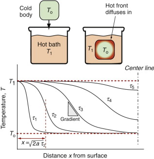
A heat exchanger transfers heat from one fluid to another while keeping the fluids physically separated. You find them in central heating systems, power-generating plants, and cooling systems in car and marine engines. Heat is transferred most efficiently if the material separating the fluids is kept thin and if the surface area for heat conduction is large—a good solution is a tubular coil. At least one of the fluids is under pressure, so the tubes must be strong enough to withstand it. Here there is a conflict in the design: thinner walls conduct heat faster, thicker walls are stronger. How is this trade-off optimised by choosing the tube material?
Consider the idealised heat exchanger made of thin-walled tubes shown in Figure 12.16. The tubes have a given radius r, a wall thickness t (which may be varied) and must support an internal pressure of p, with a temperature difference of ΔT between the fluids. The objective is to maximise the heat transferred per unit surface area of tube wall. The heat flow rate per unit area is given by
The stress due to the internal pressure in a cylindrical thin-walled tube (Chapter 10, equation (10.7)) is

This stress must not exceed the yield strength σy of the material of which it is made, so the minimum thickness t needed to support the pressure p is

Combining equations (12.16) and (12.17) to eliminate the free variable t gives
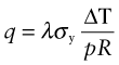
The best materials are therefore those with the highest values of the index λσy. They are the ones at the top right of the λ–σy chart of Figure 12.6—metals and certain ceramics. Ceramics are brittle and difficult to shape into thin-walled tubes, leaving metals as the only viable choice. The chart shows that the best of these are the alloys of copper and of aluminum. Both offer good corrosion resistance, but aluminum wins where cost and weight are to be kept low—in automotive radiators, for example. Commercial aluminum alloys used for this application are identified in Figure 12.11. They do not offer quite the highest values of λσy among the aluminum alloys—other factors are at work here. One is the continuous exposure to temperature during service, which can soften the precipitation-hardened alloys; another is that an efficient manufacturing route for thin-walled multi-channel tubing is extrusion, for which high ductility is needed.
Many aluminum alloys corrode in salt water. Marine heat exchangers use copper alloys even though they are heavier and more expensive because of their resistance to corrosion in seawater.
Insulation: thermal walls
Before 1940 few people had central heating or air-conditioning. Now most have both, and saunas and freezers and lots more. All consume power, and consuming power is both expensive and hard on the environment (Chapter 20). To save on both, it pays to insulate. Consider, as an example, the oven of Figure 12.17. The power lost per m2 by conduction through its wall is
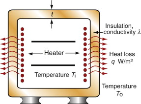
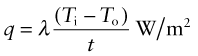
where t is the thickness of the insulation, T0 is the temperature of the outside and Ti that of the inside. For a given wall thickness t the power consumption is minimised by choosing materials with the lowest possible λ. The chart of Figure 12.6 shows that these are foams, largely because they are about 95% gas and only 5% solid. Polymer foams are usable up to about 170 °C; above this temperature even the best of them lose strength and deteriorate. When insulating against heat, then, there is an additional constraint that must be met: that the material has a maximum service temperature Tmax that lies above the planned temperature of operation. Metal foams are usable to higher temperatures but they are expensive and—being metal—they insulate less well than polymers. For high temperatures ceramic foams are the answer. Low-density firebrick is relatively cheap, can operate up to 1000 °C and is a good thermal insulator. It is used for kiln and furnace linings.
Using heat capacity: storage heaters
The demand for electricity is greater during the day than during the night. It is not economic for electricity companies to reduce output, so they seek instead to smooth demand by charging less for off-peak electricity. Storage heaters exploit this, using cheap electricity to heat a large block of material from which heat is later extracted by blowing air over it.
Storage heaters also fill other more technical roles. When designing supersonic aircraft or re-entry vehicles, it is necessary to simulate the conditions they encounter—hypersonic air flow at temperatures up to 1000 °C. The simulation is done in wind tunnels in which the air stream is heated rapidly by passing it over a previously heated thermal mass before it hits the test vehicle, as in Figure 12.18. This requires a large mass of heat-storage material, and to keep the cost down the material must be cheap. The objective, both for the home heater and for the wind tunnel, is to store as much heat per unit cost as possible.
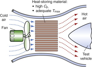
Figure 12.18 A wind tunnel with storage heating. The thermal mass is pre-heated, giving up its heat to the air blast when the fan is activated.
The energy stored in a mass m of material with a heat capacity Cp when heated through a temperature interval ΔT is
The cost of mass m of material with a cost per kg of Cm is
Thus, the heat stored per unit material cost is

The best choice of material is simply that with the largest heat capacity, Cp, and lowest price, Cm. There is one other obvious constraint: the material must be able to tolerate the temperature to which it will be heated—say, Tmax > 150 °C for the home heater, Tmax > 1000 °C for the air tunnel. It is hard to do this selection with the charts provided here, but easy to do it with the CES software: apply the limit on Tmax then use the index

to isolate the cheapest candidates. You will find that the best choice for the home heater is concrete (cast to a shape that provides some air channels). For the wind tunnel, in which temperatures are much higher, the best choice is a refractory brick with air channels for rapid heat extraction.
Using phase change: thermal buffers
When materials vaporise, or melt, or change their crystal structure while remaining solid (all of which are known as ‘phase changes’), many things happen, and they can be useful. They change in volume. If solid, they may change in shape. And they absorb or release heat, the latent heat L (J/kg) of the phase change, without changing temperature.
Suppose you want to keep something at a fixed temperature without external power. Perfect insulation is not just impractical, it is impossible. But—if keeping things warm is the problem—the answer is to surround them by a liquid that solidifies at the temperature that you want to maintain. As it solidifies it releases its latent heat of fusion, holding the temperature precisely at its solidification temperature (i.e. its melting point) until all the liquid is solid—it is the principle on which some food warmers and ‘back-woods’ hand warmers work. The reverse is also practical: using latent heat of melting to keep things cool. For this, choose a solid that melts, absorbing latent heat, at the temperature you want to maintain—‘cool bag’ inserts for holiday travel work in this way. In both cases, change of phase is used as a thermal buffer.
Shape-memory and super-elastic materials
Almost all materials expand on heating and shrink on cooling. Some few have a different response, one that comes from a solid-state phase change. Shape-memory materials are alloys based on titanium or nickel that can, while still solid, exist in two different crystal configurations with different shapes, called allotropes. If you bend the material it progressively changes structure from the one allotrope to the other, allowing enormous distortion. Shape-memory alloys have a critical temperature. If below this critical temperature, the distorted material just stays in its new shape. Warm it up and, at its critical temperature, the structure reverts to the original allotrope and the sample springs back to its original shape. This has obvious application in fire alarms, sprinkler systems and other temperature-controlled safety systems, and they are used for all of these.
But what if room temperature is already above this critical temperature? Then the material does not sit waiting for heat, but springs back to its original shape as soon as released, just as if it were elastic. The difference is that the phase change allowed distortions that are larger, by a factor of 100 or more, than straightforward elasticity without the phase change. The material is super-elastic. It is just what is needed for eyeglass frames that get sat on and otherwise mistreated, or springs that must allow very large displacements at constant restoring force—and these, indeed, are the main applications for these materials.
12.7 Summary and conclusions
- A specific heat, Cp: the amount of energy it takes to heat unit mass by unit temperature.
- A thermal expansion, α: the change in its dimensions with change of temperature.
- A thermal conductivity λ and thermal diffusivity a: the former characterising how fast heat is transmitted through the solid, the latter how long it takes for the temperature, once perturbed, to settle back to a steady pattern.
- Characteristic temperatures of its changes of phase or behavior: for a crystalline solid, its melting point Tm, and for noncrystalline solids, a glass transition temperature Tg; for design in all materials, an empirical temperature may be defined, the maximum service temperature Tmax, above which, for reasons of creep or degradation, continuous use is impractical.
- Latent heats of melting and of vaporisation: the energy absorbed or released at constant temperature when the solid melts or evaporates.
These properties can be displayed as material property charts—examples of which are utilised in this chapter. The charts illustrate the great range of thermal properties and the ways they are related. To explain these we need an understanding of the underlying physics. The key concepts are that thermal energy is atomic-level vibration, that increasing the amplitude of this vibration causes expansion, and that the vibrations propagate as phonons, giving conduction. In metals the free electrons—the ones responsible for electrical conduction—also transport heat, and they do so more effectively than phonons, giving metals their high thermal conductivities. Thermal properties are manipulated by interfering with these processes: alloying to scatter phonons and electrons; foaming to dilute the solid with low-conductivity, low-specific-heat gases.
The thermal response can be a problem in design—thermal stress, for instance, causes cracking. It can also be useful—thermal distortion can be used for actuation or sensing. It is the specific heat that makes an oven take 15 minutes to warm up, but it also stores heat in a way that can be recovered on demand. Good thermal conduction is not what you want in a coffee cup, but when it cools the engine of your car or the chip in your computer it is a big help.
This chapter has been about the thermal properties of materials. Heat, as we have said, also changes other properties, mechanical and electrical. We look more deeply into that in Chapter 13.
Cottrell A.H. The Mechanical Properties of Matter 1964 Wiley London, UK ISBN 90-247-2580-1. (A standard, well-documented introduction to the intricacies of fracture mechanics.)
Hollman J.P. Heat Transfer 5th ed.) 1981 McGraw-Hill New York, USA ISBN 0-7131-3515-8. (An introduction to fracture mechanics and testing for both static and cyclic loading.)
Tabor D. Gases, Liquids and Solids 1969 Penguin Books Harmondsworth, UK ISBN 0-471-63589-8. (A readable and detailed coverage of deformation, fracture and fatigue.)
12.9 Exercises
- Exercise E12.1 Define specific heat. What are its units? How would you calculate the specific heat per unit volume from the specific heat per unit mass? If you wanted to select a material for a compact heat storing device, which of the two would you use as a criterion of choice?
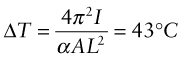
- Exercise E12.2 What two metals would you choose from the λ–a chart of Figure 12.5 to maximise the thermal displacement of a bimetallic strip actuator? If the bimetallic strip has thickness 2 mm and average thermal diffusivity a of 5 × 10⁻⁵/°C, how long will it take to respond when the temperature suddenly changes?
- Exercise E12.3 A new alloy has a density of 7380 kg/m3. Its specific heat has not yet been measured. How would you make an approximate estimate of its value in the normal units of J/kg.K? What value would you then report?
- Exercise E12.4 The same new alloy of the last exercise has a melting point of 1540 K. Its thermal expansion coefficient has not yet been measured. How would you make an approximate estimate of its value? What value would you then report?
- Exercise E12.5 Interior wall insulation should insulate well, meaning low thermal conductivity, λ, but require as little heat as possible to warm up when the central heating system is turned on (if the wall absorbs heat the room stays cold). Use the λ–a chart of Figure 12.5 to find the materials that do this best (the contours will help).
Exercise E12.6 You notice that the ceramic coffee mugs in the office get too hot to hold about 10 seconds after pouring in the hot coffee. The wall thickness of the cup is 2 mm.
- (a) What, approximately, is the thermal diffusivity of the ceramic of the mug?
- (b) Given that the volume specific heat of solids, ρCp, is more or less constant at 2 × 10⁶ J/m3 · K, what approximately is the thermal conductivity of the cup material?
- (c) If the cup were made of a metal with a thermal diffusivity of 2 × 10⁻⁵ m2/s, how long could you hold it?
- Exercise E12.7 A structural material is sought for a low-temperature device for use at –20 °C that requires high strength but low thermal conductivity. Use the λ–σy chart of Figure 12.6 to suggest two promising candidates (reject ceramics on the grounds that they are too brittle for structural use in this application).
- Exercise E12.8 A material is needed for a small, super-efficient pressurised heat exchanger. The text explained that the index for this application is M = λσy. Plot contours of this index onto a copy of the λ–σy chart of Figure 12.6 and hence find the two classes of materials that maximise M.
12.10 Exploring design with CES (use Level 2, Materials, for all selections)
Exercise E12.9 Use the ‘Search’ facility of CES to find materials for:
- Exercise E12.10 The analysis of storage heaters formulated the design constraints for the heat-storage material, which can be in the form of a particle bed or a solid block with channels to pass the air to be heated. Use the selector to find the best materials. Here is a summary of the design requirements. List the top six candidates in ranked order.
| Function | •Storage heater |
| Constraints | •Maximum service temperature >150 °C |
| •Non-flammable (a durability rating) | |
| Objective | •Maximise specific heat/material cost, Cp/Cm |
| Free variables | •Choice of material |
- Exercise E12.11 The requirements for a material for an automobile radiator, described in the text, are summarised in the table. Use CES to find appropriate materials to make them. List the top four candidates in ranked order.
| Function | •Automobile heat exchanger |
| Constraints | •Elongation >10% |
| •Maximum use temperature >180 °C | |
| •Price <5 $/kg | |
| •Durability in fresh water = very good | |
| Objective | •Maximise thermal conductivity × yield strength, λσy |
| •Wall thickness, t | |
| Free variables | •Choice of material |
- Exercise E12.12 A structural material is sought for a low-temperature device for use at –20 °C that requires high tensile strength σts but low thermal conductivity λ. For reasons of damage tolerance the fracture toughness K1c must be greater than 15 MPa.m1/2. Apply the constraint on K1c using a ‘Limit’ stage, then make a chart with σts on the x-axis and λ on the y-axis, and observe which materials best meet the requirements. Which are they?
- Exercise E12.13 Interior wall insulation should insulate well, meaning low thermal conductivity, λ, but require as little heat as possible to warm up to the desired room temperature when the central heating system is turned on—that means low specific heat. The thickness of the insulation is almost always limited by the cavity space between the inner and outer wall, so it is the specific heat per unit volume, not per unit mass, that is important here. To be viable the material must have enough stiffness and strength to support its own weight and be easy to install—take that to mean a modulus E > 0.01 GPa and a strength σy > 0.1 MPa. Make a selection based on this information. List the materials you find that best meet the design requirements.
- Exercise E12.14 Here is the gist of an email one of the authors received as this chapter was being written. ‘We manufacture wood-burning stoves and fireplaces that are distributed all over Europe. We want to select the best materials for our various products. The important characteristics for us are: specific heat, thermal conductivity, density … and price, of course. What can your CES software suggest?’
Form your judgement about why these properties matter to them. Rank them, deciding which you would see as constraints and which as the objective. Consider whether there are perhaps other properties they have neglected. Then—given your starting assumptions of just how these stoves are used—use CES to make a selection. Justify your choice.
There is no ‘right’ answer to this question—it depends on the assumptions you make. The essence is in the last sentence of the last paragraph: justify your choice.
12.11 Exploring the science with CES Elements
- Exercise E12.15 The text says that materials expand about 2% between 0 K and their melting point. Use CES Elements to explore the truth of this by making a bar chart of the expansion at the melting point, αTm/106 (the 106 is to correct for the units of α used in the database).
- Exercise E12.16 When a solid vaporises, the bonds between its atoms are broken. You might then expect that latent heat of vaporisation, Lv, should be nearly the same as the cohesive energy, Hc, since it is the basic measure of the strength of the bonding. Plot one against the other, using CES Elements. How close are they?
- Exercise E12.17 When a solid melts, some of the bonds between its atoms are broken, but not all—liquids still have a bulk modulus, for example. You might then expect that the latent heat of melting, Lm, should be less than the cohesive energy, Hc, since it is the basic measure of the strength of the bonding. Plot one against the other, using CES Elements (Lm is called the heat of fusion in the database). By what factor is Lm less than Hc? What does this tell you about cohesion in the liquid?
Exercise E12.18 The latent heat of melting (heat of fusion), Lm, of a material is said to be about equal to the heat required to heat it from absolute zero to its melting point, CpTm, where Cp is the specific heat and Tm is the absolute melting point. Make a chart with Lm on one axis and CpTm on the other. To make the comparison right we have to change the units of Lm in making the chart to J/kg instead of kJ/mol. To do this multiply Lm by
- using the ‘Advanced’ facility when defining axes in CES. Is the statement true?
- Exercise E12.19 The claim was made in the text that the modulus E is roughly proportional to the absolute melting point Tm. If you use CES Elements to explore this correlation you will find that it is not, in fact, very good (try it). That is because Tm and E are measured in different units and, from a physical point of view, the comparison is meaningless. To make a proper comparison, we use instead kBTm and EΩ, where kB is Boltzmann’s (1.38 × 10⁻²³ J/K) constant and Ωm3/atom is the atomic volume. These two quantities are both energies, the first proportional to the thermal energy per atom at the melting point and the second proportional to the work to elastically stretch an atomic bond. It makes better sense, from a physical standpoint, to compare these.
- Make a chart for the elements with kBTm on the x-axis and EΩ on the y-axis to explore how good this correlation is. Correlations like these (if good) that apply right across the periodic table provide powerful tools for checking data, and for predicting one property (say, E) if the other (here, Tm) is known. Formulate an equation relating the two energies that could be used for these purposes.
Exercise E12.20 Above the Debye temperature, the specific heat is predicted to be 3R, where R is in units of kJ/kmol.K. Make a plot for the elements with Debye temperature on the x-axis and specific heat in these units on the y-axis to explore this. You need to insert a conversion factor because of the units. Here it is, expressed in the units contained in the database:
- Form this quantity, dividing the result by R = 8.314 kJ/kmol.K, and plot it against the Debye temperature. The result should be 3 except for materials with high Debye temperatures. Is it? Fit a curve by eye to the data. At roughly what temperature does the drop-off first begin?
Exercise E12.21 Explore the mean free path of phonons, ℓm in the elements using equation (12.10) of the text. Inverting it gives
in which the speed of sound
 . Use the ‘Advanced’ facility when defining the axes in CES to make a bar chart of ℓm for the elements. Which materials have the longest values? Which have the shortest?

1Benjamin Thompson (1753–1814), later Lord Rumford, while in charge of the boring of cannons at the Watertown Arsenal near Boston, Mass., noted how hot they became and formulated the ‘mechanical equivalent of heat’—what we now call the heat capacity.
2Sadi Nicolas Léonhard Carnot (1796–1832), physicist and engineer, formulator of the Carnot cycle and the concept of entropy, the basis of the optimisation of heat engines. He died of cholera, a fate most physicists today, mercifully, are spared.
3William Thompson, Lord Kelvin (1824–1907), Scottish mathematician who contributed to many branches of physics; he was known for a self-confidence that led him to claim (in 1900) that there was nothing more to be discovered in physics—he already knew it all.
4James Joule (1818–1889), English physicist, who, motivated by theological belief, sought to establish the unity of the forces of nature. His demonstration of the equivalence of heat and mechanical work did much to discredit the caloric theory.
5James Watt (1736–1819), instrument maker and inventor of the condenser steam engine (the idea came to him while ‘walking on a fine Sabbath afternoon’), which he doggedly developed. Unlike so many of the characters footnoted in this book, Watt, in his final years, was healthy, happy and famous.
6Baron Jean Baptiste Joseph Fourier (1768–1830), mathematician and physicist; he nearly came to grief during the French Revolution but survived to become one of the savants who accompanied Napoleon Bonaparte in his conquest of Egypt.
7Albert Einstein (1879–1955), Patent Officer, physicist and campaigner for peace, one of the greatest scientific minds of the 20th century; he was forced to leave Germany in 1933, moving to Princeton, NJ, where his influence on US defence policy was profound.
8Peter Debye (1884–1966), Dutch physicist and Nobel Prize winner, did much of his early work in Germany until in 1938, harassed by the Nazis, he moved to Cornell, NY, where he remained until his death.
9Ludwig Boltzmann (1844–1906), born and worked in Vienna at a time when that city was the intellectual center of Europe; his childhood interest in butterflies evolved into a wider interest in science, culminating in his seminal contributions to statistical mechanics.