
3
Workings of the Federated Learning System
This chapter will provide an overview of the architecture, procedure flow, sequence of messages, and basics of model aggregation of the federated learning (FL) system. As discussed in Chapter 2, What Is Federated Learning?, the conceptual basics of the FL framework are quite simple and easy to understand. However, the real implementation of the FL framework needs to come with a good understanding of both AI and distributed systems.
The content of this chapter is based on the most standard foundation of FL systems, which is used in hands-on exercises later in the book. First, we will introduce the building blocks of FL systems, such as an aggregator with an FL server, an agent with an FL client, a database server, and communication between these components. The architecture introduced in this chapter is designed in a decoupled way so that further enhancement to the system will be relatively easier than with an FL system that contains everything on one machine. Then, an explanation of the flow of the operation of FL from initialization to aggregation will follow.
Finally, we will examine the way an FL system is scaled with a horizontal design of decentralized FL setups.
This chapter covers the following topics:
- FL system architecture
- Understanding the FL system flow – from initialization to continuous operation
- Basics of model aggregation
- Furthering scalability with horizontal design
FL system architecture
FL systems are distributed systems that are dispersed into servers and distributed clients. Here, we will define a representative architecture of an FL system with the following components: an aggregator with an FL server, an agent with an FL client, and a database:
- Cluster aggregator (or aggregator): A system with an FL server that collects and aggregates machine learning (ML) models that are trained at multiple distributed agents (defined shortly) and creates global ML models that are sent back to the agents. This system serves as a cluster aggregator, or more simply, an aggregator of FL systems.
- Distributed agent (or agent): A distributed learning environment with an FL client such as a local edge device, mobile application, tablet, or any distributed cloud environment where ML models are trained in a distributed manner and sent to an aggregator. The agent can be connected to an FL server of the aggregator through the FL client-side communications module. The FL client-side codes contain a collection of libraries that can be integrated into the local ML application, which is designed and implemented by individual ML engineers and data scientists.
- Database server (or database): A database and its server to store the data related to the aggregators, agents, and global and local ML models and their performance metrics. The database server handles the incoming queries from the aggregators and sends the necessary data back to the aggregators. Agents do not have to be connected to the database server directly for the simplicity of the FL system design.
Figure 3.1 shows the typical overall architecture consisting of a single cluster aggregator and a database server, as well as multiple distributed agents:

Figure 3.1 – Overall architecture of an FL system
One advantage of the FL system’s architecture is that users do not have to send private raw data to the server, especially that owned by a third party. Instead, they only have to send locally trained models to the aggregator. The locally trained models can be in a variety of formats such as the weights of the entire ML models, the changes of weights (gradients), or even a subset of them. Another advantage includes reducing the communication load because the users only have to exchange models that are usually much lighter than raw data.
Cluster aggregators
A cluster aggregator consists of an FL server module, FL state manager module, and model aggregation module, as in Figure 3.1. We just call a cluster aggregator with an FL server an aggregator. While these modules are the foundation of the aggregator, advanced modules can be added to ensure further security and flexibility of the aggregation of ML models. Some of the advanced modules are not implemented in the simple-fl GitHub repository provided with this book with exercises because the main purpose of this book is to understand the basic structure and system flow of the FL system. In the aggregator system, the following modules related to the FL server, the state manager of FL, and model aggregation are the keys to implementing the aggregator-side functionalities.
- FL server module: There are three primary functionalities for the FL server module, which include the communication handler, system configuration handler, and model synthesis routine:
- Communication handler: Serves as a module of the aggregator that supports communications with agents and the database. Usually, this module accepts polling messages from agents and sends responses back to them. The types of messages they receive include the registration of agents themselves with secure credentials and authentication mechanisms, the initialization of the ML model that serves as an initial model for the future aggregation process, confirmation about whether or not agents participate in a round, and local ML models that are retrained at distributed agents such as mobile devices and local edge machines. The communication handler can also query the database server in order to access the system data and ML models in the database, as well as push and store this data and those models once the aggregator receives or creates new models. This module can utilize HTTP, WebSocket, or any other communication framework for its implementation.
- System configuration handler: Deals with the registration of agents and tracking the connected agents and their statuses. The aggregator needs to be aware of the connections and registration statuses of the agents. If the agents are registered with an established authentication mechanism, they will accept the messages and process them accordingly. Otherwise, this module will go through the authentication process, such as validating the token sent from the agent, so that next time this agent is connected to the FL server, the system will recognize the agent properly.
- Model synthesis routine: Supports checking the collection status of the local ML models and aggregating them once the collection criteria are satisfied. Collection criteria include the number of local models collected by the connected agents. For example, aggregation can happen when 80% of the connected agents send the trained local models to the aggregator. One of the design patterns to do so is to periodically check the number of ML models uploaded by the agents, which keep running while the FL server is up and running. The model synthesis routine will access the database or local buffer periodically to check the status of the local model collection and aggregate those models, to produce the global model that will be stored in the database server and sent back to the agents.
- FL state manager: A state manager keeps track of the state information of an aggregator and connected agents. It stores volatile information for an aggregator, such as local and global models delivered by agents, cluster models pulled from the database, FL round information, or agents connected to the aggregator. The buffered local models are used by the model aggregation module to generate a global model that is sent back to each active agent connected to the aggregator.
- Model aggregation module: The model aggregation module is a collection of the model aggregation algorithms introduced in the Basics of model aggregation section in this chapter and Chapter 7, Model Aggregation, in further depth. The most typical aggregation algorithm is federated averaging, which averages the weights of the collected ML models, considering the number of samples that each model has used for its local training.
Distributed agents
A distributed agent consists of an FL client module that includes the communication handler and client libraries as well as local ML applications connected to the FL system through the FL client libraries:
- FL client module: There are primarily four key functionalities for the FL client module, which include a communication handler, agent participation handler, model exchange routine, and client libraries:
- Communication handler: Serves as a channel to communicate with the aggregator that is assigned to the agent. The message sent to the aggregator includes the registration payload of the agent itself and an initial model that will be the basis of aggregated models. The message also contains locally trained models together with the performance data of those models. This module supports both push and polling mechanisms and can utilize HTTP or WebSocket frameworks for its implementation.
- FL participation handler: Deals with the agent participation in the FL process and cycle by sending an aggregator a message including the agent information itself to be registered in the FL platform and initialize the FL process if needed. The response message will set the agent up for the continuous and ongoing FL process and often includes the most updated global model for the agent to utilize and train locally.
- Model exchange routine: Supports a synchronizing functionality that constantly checks whether a new global model is available or not. If the new global model is available, this module downloads the global model from the aggregator and the global model replaces the local model if needed. This module also checks the client state and sends the retrained model if the local training process is done.
- Client libraries: Include administrative libraries and general FL client libraries:
- The administrative libraries are used when registering the initial model that will be used by other agents. Any configuration changes for FL systems can be also requested by administrative agents that have higher control capabilities.
- General FL client libraries provide basic functionalities such as starting FL client core threads, sending local models to an aggregator, saving models in some specific location on the local machine, manipulating the client state, and downloading the global models. This book mainly talks about this general type of library.
- Local ML engine and data pipelines: These parts are designed by individual ML engineers and scientists and can be independent of the FL client functionalities. This module has an ML model itself that can be put into play immediately by the user for potentially more accurate inference, a training and testing environment that can be plugged into the FL client libraries, and for the implementation of data pipelines. While the aforementioned module and libraries can be generalized and provided as application programming interfaces (APIs) or libraries for any ML applications, this module is unique depending on the requirements of AI applications to be developed.
Database servers
A database server consists of a database query handler and a database, as storage. The database server can reside on the server side, such as on the cloud, and is tied closely to aggregators, while the recommended design is to separate this database server from aggregator servers to decouple the functionalities to enhance the system’s simplicity and resilience. The functionality of the database query handler and sample database tables are as follows:
- Database query handler: Accepts the incoming requests from an aggregator and sends the requested data and ML models back to the aggregator.
- Database: Stores all the related information to FL processes. We list some potential entries for the database here:
- Aggregator information: This aggregator-related information includes the ID of the aggregator itself, the IP address and various port numbers, system registered and updated times, and system status. In addition, this entry can include model aggregation-related information, such as the round of FL and its information and aggregation criteria.
- Agent information: This agent-related information includes the ID of the agent itself, the IP address and various port numbers, system registered and updated times, and system status. This entry can also contain the opt-in/out status that is used for synchronous FL (explained in the Synchronous and asynchronous FL section in this chapter) and a flag to record whether the agent has been a bad actor in the past (for example, involved in poisoning attacks, or very slow at returning results).
- Base model information: Base model information is used for the registration of initial ML models whose architecture and information are used for the entire process of FL rounds.
- Local models: The information of local models includes the model ID that is unique to individual ML models, generated time of the model, agent ID that uploaded the model, aggregator ID that received the model from the agent, and so on. Usually, the model ID is uniquely mapped to the location of the actual ML model file that can be stored in the database server or in some cloud storage services such as S3 buckets of Amazon Web Services, and so on.
- Cluster global models: The information of the cluster global models is similar to what local models could record in the database including the model ID, aggregator ID, generated time of the model, and so on. Once the aggregated model is created by an aggregator, the database server will accept the global models and store them in the database server or any cloud storage services. Any global model can be requested by an aggregator.
- Performance data: The performance of the local and global models can be tracked, as metadata attached to those models. This performance data will be used to ensure that the aggregated model performs well enough before it is actually deployed to the user ML application.
Note
In the code sample of the simple-fl repository, only the database tables related to the local models and cluster models are covered to simplify the explanation of the entire FL process.
Now that the basic architecture of the FL system has been introduced, next, we will talk about how to enhance the FL system’s architecture if the computation resources are limited on the agent-side devices.
Intermediate servers for low computational agent devices
Sometimes, the computational capability of local user devices is limited – ML training may be difficult in those devices, but inference or predictions can be made possible by just downloading the global model. In these cases, an FL platform may be able to set up an additional intermediate server layer, such as with smartphones, tablets, or edge servers. For example, in a healthcare AI application, users manage their health information on their smart watches, which can be transferred to their smart tablets or synched with laptops. In those devices, it is easy to retrain ML models and integrate the distributed agent functionalities.
Therefore, the system architecture needs to be modified or redesigned depending on the applications into which the FL system is integrated, and the concept of intermediate servers can be applied using distributed agents to realize FL processes. We do not have to modify the interactions and communication mechanisms between the aggregators and the intermediate servers. Just by implementing APIs between the user devices and the intermediate servers, FL will be possible in most use cases.
Figure 3.2 illustrates the interaction between the aggregators, intermediate servers, and user devices:

Figure 3.2 – An FL system with intermediate servers
Now that we have learned about the basic architecture and components of an FL system, let us look into how an FL system operates in the following section.
Understanding the FL system flow – from initialization to continuous operation
Each distributed agent belongs to an aggregator that is managed by an FL server, where ML model aggregation is conducted to synthesize a global model that is going to be sent back to the agents. An agent uses its local data to train an ML model and then uploads the trained model to the corresponding aggregator. The concept sounds straightforward, so we will look into a bit more detail to realize the entire flow of those processes.
We also define a cluster global model, which we simply call a cluster model or global model, which is an aggregated ML model of local models collected from distributed agents.
Note
In the next two chapters, we will guide you on how to implement the procedure and sequence of messages discussed in this chapter. However, some of the system operation perspectives, such as an aggregator or agent system registration in the database, are not introduced in the code sample of the simple-fl repository in order to simplify the explanation of the entire FL process.
Initialization of the database, aggregator, and agent
The sequence of the initialization processes is quite simple. The initialization and registration processes need to happen in the order of database, aggregator, and agents. The overall registration sequence of an aggregator and an agent with a database is depicted in Figure 3.3 as follows:

Figure 3.3 – The process of aggregator and agent registration in the database server
Here is the initialization and registration procedure of each component in the FL system:
- Database server initialization: The first step of the operation of an FL system is to initiate the database server. There are some simple frameworks that are provided by multiple organizations that do not include databases or database servers. However, in order to maintain the process of federating the ML models, it is recommended that you use a database, even a lightweight one such as an SQLite database.
- Aggregator initialization and registration: An aggregator should be set up and running before any agents start running and uploading the ML models. When the aggregator starts running and first gets connected to the database server, the registration process happens automatically by also checking whether the aggregator is safe to be connected. If it fails to go through the registration process, it receives the registration failure message sent back from the database. Also, in case the aggregator is trying to connect to the database again after losing the connection to the database, the database server always checks whether the aggregator has already been registered or not. If this is the case, the response from the database server includes the system information of the registered aggregator so that the aggregator can start from the point where it left off. The aggregator may need to publish an IP address and port number for agents to be connected if it uses HTTP or WebSocket.
- Agent initialization and registration: Usually, if an agent knows the aggregator that the agent wants to connect to, the registration is similar to how an aggregator connects to a database server. The connection process should be straightforward enough to just send a participation message to that aggregator using an IP address, the port number of the aggregator (if we are using some frameworks such as HTTP or WebSocket), and an authentication token. In case the agent is trying to connect to the aggregator again after losing the connection to the aggregator, the database server always checks whether the agent already has been registered or not. If the agent is already registered, the response from the database server includes the system information of the registered agent so that the agent can start from the point where it was disconnected from the aggregator.
In particular, when it receives the participation message from the agent, the aggregator goes through the following procedure, as in Figure 3.4. The key process after receiving the participation request is (i) checking whether the agent is trusted or not, or whether the agent is already registered or not, and (ii) checking whether the initial global model is already registered or not. If (i) is met, the registration process keeps going. If the (initial) global model is already registered, the agent will be able to receive the global model and start using that global model for the local training process on the agent side.
The agent participation and registration process at an aggregator side is depicted in Figure 3.4:

Figure 3.4 – The registration process of an agent by an aggregator
Now that we understand the initialization and registration process of the FL system components, let us move on to the basic configuration of the ongoing FL process, which is about uploading the initial ML model.
Initial model upload process by initial agent
The next step in running an FL process is to register the initial ML model whose architecture will be used in the entire and continuous process of FL by all the aggregators and agents. The initial model can be distributed by the company that owns the ML application and FL servers. They’ll likely provide the initial base model as part of the aggregator configuration.
We call the initial ML model used as a reference for model aggregation a base model. We also call the agent that uploads the initial base model an initial agent. The base model info could include the ML model itself as well as the time it was generated and the initial performance data. That being said, the process of initializing the base model can be seen in Figure 3.5:

Figure 3.5 – Base model upload process for the initial agent
Now, the FL process is ready to be conducted. Next, we will learn about the FL cycle, which is a very core part of the FL process.
Overall FL cycle and process of the FL system
In this section, we will only give an example with a single agent and aggregator, but in real cases and operations, the agent environments are various and dispersed into distributed devices. The following is the list of the processes for how the local models are uploaded, aggregated, stored, and sent back to agents as a global model:
- The agents other than the initial agent will request the global model, which is an updated aggregated ML model, in order to deploy it to their own applications.
- Once the agent gets the updated model from the aggregator and deploys it, the agent retrains the ML model locally with new data that is obtained afterward to reflect the freshness and timeliness of the data. An agent can also participate in multiple rounds with different data to absorb its local examples and tendencies. Again, this local data will not be shared with the aggregator and stays local to the distributed devices.
- After retraining the local ML model (which, of course, has the same architecture as the global or base model of the FL), the agent calls an FL client API to send the model to the aggregator.
- The aggregator receives the local ML model and pushes the model to the database. The aggregator keeps track of the number of collected local models and will keep accepting the local models as long as the federation round is open. The round can be closed with any defined criteria, such as the aggregator receiving enough ML models to be aggregated. When the criteria are met, the aggregator aggregates the local models and produces an updated global model that is ready to be sent back to the agent.
- During that process, agents constantly poll the aggregator on whether the global model is ready or not, or in some cases, the aggregator may push the global model to the agents that are connected to the aggregator, depending on the communications system design and network constraints. Then, the updated model is sent back to the agent.
- After receiving the updated global model, the agent deploys and retrains the global model locally whenever it is ready. The whole process described is repeated until the termination criteria are met for the FL to end. In some cases, there are no termination conditions to stop this FL cycle and retraining process so that the global model constantly keeps learning about the latest phenomena, current trends, or user-related tendencies. FL rounds can just be stopped manually in preparation for some evaluation before a rollout.
Figure 3.6 shows the overall process of how FL is continuously conducted between an agent, an aggregator, and a database typically:

Figure 3.6 – Overview of the continuous FL cycle
Now that we understand the overall procedure of the FL process, we will look into the different round management approaches in the FL process next: synchronous FL and asynchronous FL.
Synchronous and asynchronous FL
When the model aggregation happens at the aggregator, there are multiple criteria related to how many local models it needs to collect from which agents. In this section, we will briefly talk about the differences between synchronous and asynchronous FL, which have been discussed in a lot of literature, such as https://iqua.ece.toronto.edu/papers/ningxinsu-iwqos22.pdf, so please refer to it to learn about these concepts further.
Synchronous FL
Synchronous FL requires the aggregator to select the agents that need to send the local models for each round in order to proceed with the model aggregation. This synchronous FL approach is simple to design and implement and suitable for FL applications that require a clear selection of agents. However, if the number of agents becomes too large, the aggregator may have to wait for a long time to wrap up the current round, as the computational capability of the agents could vary and some of them may have problems uploading or fail to upload their local models. Thus, some of the agents can become slow or totally dysfunctional when sending their models to the aggregator. These slow agents are known as stragglers in distributed ML, which motivates us to use the asynchronous FL mode.
Asynchronous FL
Asynchronous FL does not require the aggregator to select the agents that have to upload their local models. Instead, it opens the door for any trusted agents to upload the model anytime. Furthermore, it is fine to wrap up the federation round whenever the aggregator wants to generate the global model, with or without criteria such as the minimum number of local models that needs to be collected, or some predefined interval or deadline for which the aggregator needs to wait to receive the local models from the agents until the aggregation for that round happens. This asynchronous FL approach gives the FL system much more flexibility for model aggregation for each FL round, but the design may be more complicated than the simple synchronous aggregation framework.
When managing the FL rounds, you need to consider the practicalities of running rounds, such as scheduling and dealing with delayed responses, the minimum levels of participation required, the details of example stores, using the downloaded or trained models for improved inference in the applications on the edge devices, and dealing with bad or slow agents.
We will look into the FL process and procedure flow next, focusing on the aggregator side.
The aggregator-side FL cycle and process
An aggregator has two threads running to accept and cache the local models and aggregate the collected local ML models. In this section, we describe those procedures.
Accepting and caching local ML models
The aggregator side process of accepting and caching local ML models is depicted in Figure 3.7 and explained as follows:
- The aggregator will wait for a local ML model to be uploaded by an agent. This method sounds like asynchronous FL. However, if the aggregator has already decided which agents to accept models from, it just needs to exclude the model uploads sent by undesired agents. Some other system or module may have already told the undesired agents not to participate in the round as well.
- Once an ML model is received, the aggregator checks whether the model is uploaded by the trusted agents or not. Also, if the agent that uploads the local model is not listed in the agents that the FL operator wants to accept, the aggregator will discard the model. Furthermore, an aggregator needs to have a mechanism to only filter the valid models – otherwise, there is a risk of poisoning the global model and messing up the entire FL process.
- If the uploaded local ML model is valid, the aggregator will push the model to the database. If the database resides on a different server, the aggregator will package the model and send it to the database server.
- While the uploaded models are stored in the database, they should be buffered in the memory of the state manager of the aggregator in an appropriate format, such as NumPy arrays.
This procedure keeps running until the termination conditions are satisfied or the operator of the FL system opts to stop the process. Figure 3.7 depicts the procedure of accepting and caching local ML models:

Figure 3.7 – Procedure for accepting and caching local ML models
Once the local ML models are accepted and cached, the FL system moves on to the next procedure: aggregating the local models.
Aggregating local ML models
The aggregator-side procedure of aggregating local ML models depicted in Figure 3.8 is as follows:
- The aggregator constantly checks whether the aggregation criteria are satisfied. The typical aggregation criteria are as follows:
- The number of local models collected so far in this FL round. For example, if the number of agents is 10 nodes, after 8 nodes (meaning 80% nodes) report the locally trained models, the aggregator starts aggregating the models.
- The combination of the number of collected models and the time that the FL round has spent. This can automate the aggregation process and prevent systems from getting stuck.
- Once the aggregation criteria are met, the aggregator starts a model aggregation process. Usually, federated averaging is a very typical but powerful aggregation method. Further explanation of the model aggregation methods is in the Basics of model aggregation section of this chapter and in Chapter 7, Model Aggregation. The aggregated model is defined as a global model in this FL round.
In a case where time for the FL round has expired and not enough agents that participated in the round have uploaded a model, the round can be abandoned or forced to conduct aggregation for the local models collected so far.
- Once the model aggregation is complete, the aggregator pushes the aggregated global model to the database. If the database resides on a different server, the aggregator will package the global model and send it to the database server.
- Then, the aggregator sends the global model to all the agents, or when the agents poll to check whether the global model is ready, the aggregator will notify the agent that the global model is ready and put it in the response message to the agents.
- After the whole process of model aggregation, the aggregator updates the number of the FL round by just incrementing it.
Figure 3.8 shows the aggregator’s process from checking the aggregation criteria to synthesizing the global model when enough models are collected:

Figure 3.8 – Model synthesis routine: aggregating local ML models
Aggregating local models to generate the global model has been explained. Now, let us look into the agent-side FL cycle, including the retraining process of the local ML models.
The agent-side local retraining cycle and process
In the distributed agent, the following state transition happens and is repeated for the continuous operation of the FL cycle:
- In the state of waiting_gm, the agent polls the aggregator to receive any updates related to the global model. Basically, a polling method is used to regularly query the updated global model. However, under some specific settings, an aggregator can push the updated global model to all agents.
- gm_ready is the state after the global model is formed by the aggregator and downloaded by the agent. The model parameters are cached in the agent device. The agent replaces its local ML model with the downloaded global model. Before completely replacing the local model with the downloaded model, the agent can check whether the output of the global model is sufficiently performant for the local ML engine. If the performance is not what is expected, the user can keep using the old model locally until it receives the global model that has the desired performance.
- Next, in the training state, the agent can locally train the model in order to maximize its performance. The trained model is saved in a local data storage where training examples are kept. The FL client libraries of the agent ascertain its readiness to manipulate the local model that can be protected with asynchronous function access.
- After the local model is trained, the agent checks whether the new global model has been sent to the agent or not. If the global model has arrived, then the locally trained ML model is discarded and goes back to the gm_ready state.
- After local training, the agent proceeds with the sending state to send the updated local model back to the aggregator, and then, the agent goes back to the waiting_gm state.
Figure 3.9 depicts the state transition of an agent to adapt and update the ML model:

Figure 3.9 – Agent-side state transition to adapt and update the ML model
Next, we touch on a model interpretation based on deviation from the baseline outputs that are used for anomaly detection and preventing model degradation.
Model interpretation based on deviation from baseline outputs
We can also provide an interpretation framework by looking at the output of each local model. The following procedure can be considered to ensure the local model is always good to use and can be deployed in production:
- Obtain the most recent ML output generated by an agent as well as a baseline output that can be a typical desired output prepared by users. The baseline output could include an average output based on the past windows or reference points defined by an operator, subject expert, or rule-based algorithm.
- The deviation between the output of the local model and the baseline output is computed.
- An anomaly or performance degradation can be detected by checking whether the deviation exceeds the operator-specified threshold. If an anomaly is detected, an alarm can be sent to an operator to indicate a fault or that the ML model is in an anomalous state.
Now that the process of the FL has been explained, let us look into the basics of model aggregation, which comprise the critical part of FL.
Basics of model aggregation
Aggregation is a core concept within FL. In fact, the strategies employed to aggregate models are the key theoretical driver for the performance of FL systems. The purpose of this section is to introduce the high-level concepts of aggregation within the context of an FL system – the underlying theory and examples of advanced aggregation strategies will be discussed in greater depth in Chapter 7, Model Aggregation.
What exactly does it mean to aggregate models?
Let’s revisit the aggregator-side cycle discussed in the Understanding the FL system flow – from initialization to continuous operation section, at the point in the process where the agents assigned to a certain aggregator have finished training locally and have transmitted these models back to this aggregator. The goal of any aggregation strategy, or any way of aggregating these models together, is to produce new models that gradually increase in performance across all of the data collected by the constituent agents.
An important point to remember is that FL is, by definition, a restricted version of the distributed learning setting, in which the data collected locally by each agent cannot be directly accessed by other agents. If this restriction were not in place, a model could be made to perform well trivially on all of the data by collecting the data from each agent and training on the joint dataset; thus, it makes sense to treat this centrally-trained model as the target model for an FL approach. At a high level, we can consider this unrestricted distributed learning scenario as aggregation before model training (where in this case, aggregation refers to combining the data from each agent). Because FL does not allow data to be accessed by other agents, we consider the scenario as aggregation after model training instead; in this context, aggregation refers to the combination of the intelligence captured by each of the trained models from their differing local datasets. To summarize, the goal of an aggregation strategy is to combine models in a way that eventually leads to a generalized model whose performance approaches that of the respective centrally trained model.
FedAvg – Federated averaging
To make some of these ideas more concrete, let’s take an initial look into one of the most well-known and straightforward aggregation strategies, known as Federated Averaging (FedAvg). The FedAvg algorithm is performed as follows: let  be the parameters of the models from
 ![]() agents, each with a local dataset size of
agents, each with a local dataset size of ![]() . Also,
. Also, ![]() is the total dataset size defined as
is the total dataset size defined as  . Then, FedAvg returns the following ML model as the aggregated model:

Essentially, we perform FedAvg over a set of models by taking the weighted average of the models, with weights proportional to the size of the dataset used to train the model. As a result, the types of models to which FedAvg can be applied are models that can be represented as some set of parameter values. Deep neural networks are currently the most notable of these kinds of models – most of the results analyzing the performance of FedAvg work with deep learning models.
It is rather surprising that this relatively simple approach can lead to generalization in the resulting model. We can visually examine what FedAvg looks like within a toy two-dimensional parameter space to observe the benefits of the aggregation strategy:
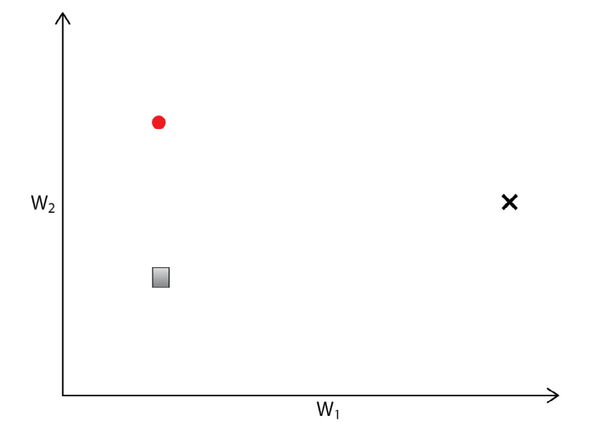
Figure 3.10 – Two-dimensional parameter space with local models from two agents (the circle and square) and a target model (the black x)
Let’s consider a case where we have two newly initialized models (the circle and square points) belonging to separate agents. The space in the preceding figure represents the parameter space of the models, where each toy model is defined by two parameters. As the models are trained, these points will move in the parameter space – the goal is to approach a local optimum in the parameter space, generally corresponding to the aforementioned centrally trained model:
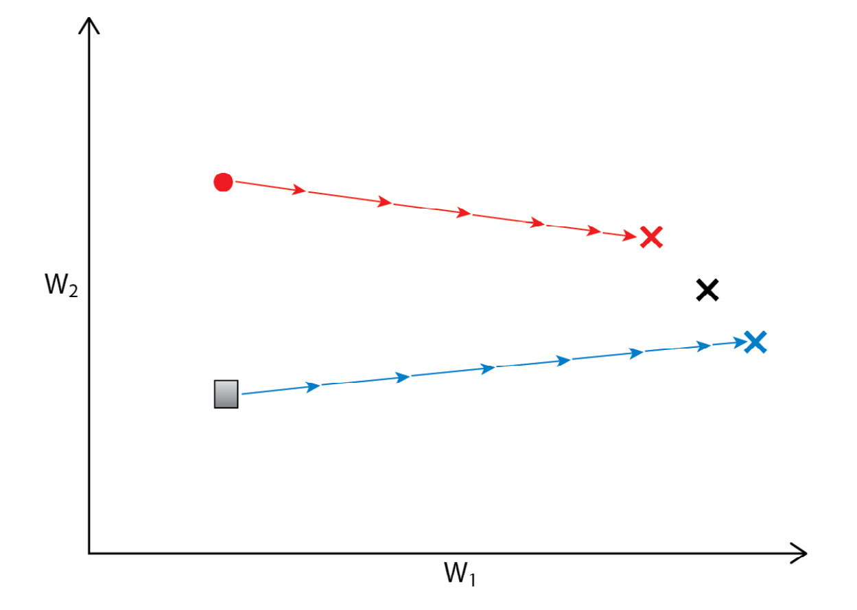
Figure 3.11 – Change in local model parameters without aggregation
Each model converges to separate dataset-specific optima (two x points from the circle and square) that do not generalize. Because each agent only has access to a subset of the data, the local optima reached by training each model locally will differ from the true local optima; this difference depends on how similar the underlying data distributions are for each agent. If the models are only trained locally, the resulting models will likely not generalize over all of the data:
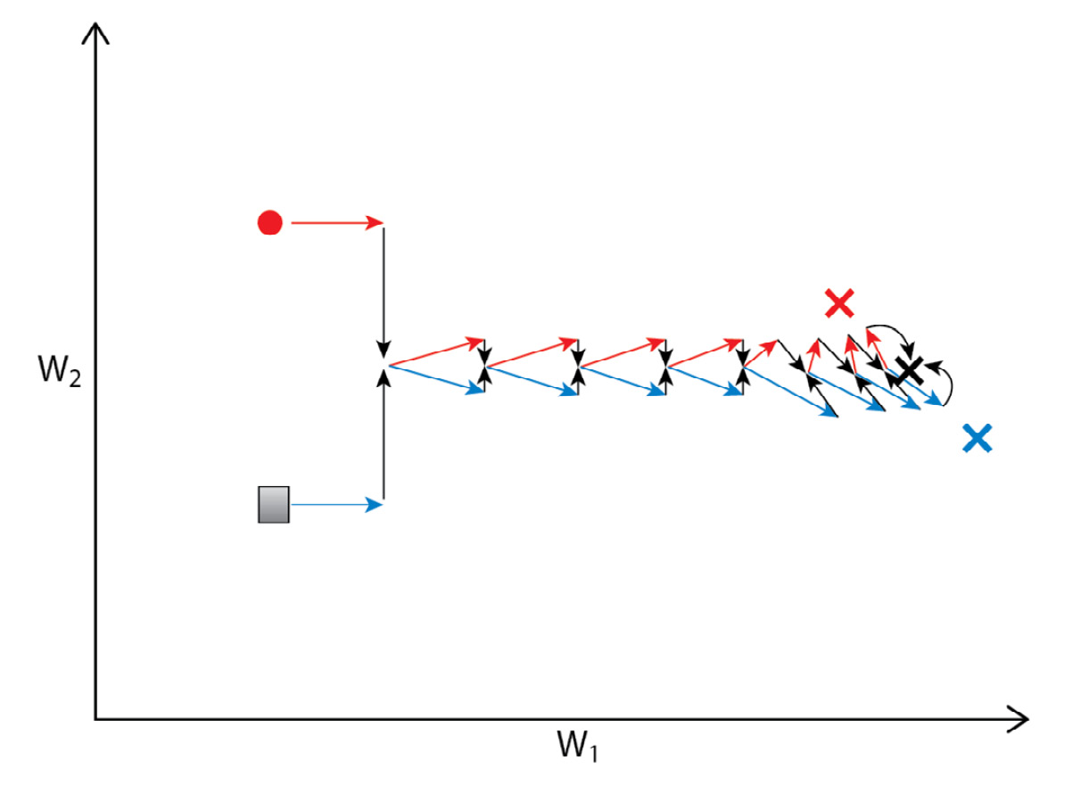
Figure 3.12 – Adding aggregation moves the local model parameters to the average for both models at each step, leading to convergence at the target model
Applying FedAvg at each movement step allows us to create an aggregate model that eventually comes close to the true local optima in the parameter space.
This example displays the basic capability of FedAvg to produce generalized models. However, working with real models (such as highly parameterized deep learning models) introduces additional complexity that is handled by FedAvg but not by simpler approaches. For example, we might wonder why we don’t simply fully train each local model and only average at the end; while this approach would work in this toy case, it has been observed that only averaging once with real models leads to poor performance across all of the data. The FedAvg process allows for a more robust way to reach the generalized model within high-dimension parameter spaces.
This section only aims to give an overview of aggregation in FL; Chapter 7, Model Aggregation, contains more detailed explanations and examples for aggregation in different scenarios.
We now understand the entire process of how the FL system works with basic model aggregation. In some applications, the FL system may have to support a huge number of agents to realize its scalability. The following section will give you some idea about how to scale more smoothly, especially with a decentralized horizontal design.
Furthering scalability with horizontal design
In this section, we will look into how to further scalability when we need to support a large number of devices and users.
There are practical cases where control, ease of maintenance and deployment, and low communication overhead are provided by centralized FL. If the number of agents is not large, it makes more sense to stick to centralized FL than decentralized FL. However, when the number of participating agents becomes quite large, it may be worth looking into horizontal scaling with a decentralized FL architecture. The latest developments of auto-scaling frameworks these days, such as the Kubernetes framework (https://kubernetes.io/), can be a nice integration with the topic that is discussed in this section, although actual integration and implementation with Kubernetes is beyond the scope of this book.
Horizontal design with semi-global model
There will be some use cases where many aggregators are needed to cluster groups of agents and create a global model on top of those many aggregators. Google uses a centralized approach for this, as in the paper Towards Federated Learning at Scale, while setting up a centralized node for managing multiple aggregators may have some resilience issues. The idea is simple: periodically aggregate all the cluster models at some central master node.
On the other hand, we can realize the decentralized way of aggregating cluster models created by multiple aggregators. The architecture for that is based on two crucial ideas:
- Model aggregation conducted among individual cluster aggregators without master nodes
- Semi-global model synthesis to aggregate cluster models generated by other aggregators
To create semi-global models, decentralized cluster aggregators exchange their aggregated cluster models with each other and approximate optimal global models. The cluster aggregators can also use a database to periodically collect other cluster models to generate the semi-global models. This framework allows for the absorption of training results from diverse sets of users dispersed across many aggregators by synthesizing the most updated global models without a master node concept.
Based on this decentralized architecture, the robustness of the entire FL system can be enhanced, as the semi-global model can be independently computed at each cluster aggregator. The FL system can be scaled further, as each cluster aggregator is responsible for creating its own semi-global model by itself – not via the master node of those aggregators – and therefore, decentralized semi-global model formation comes with resiliency and mobility.
We can even decouple the database that stores the uploaded local models, cluster global models, and semi-global models. By introducing a distributed database into the FL system, the entire system could be made more scalable, resilient, and secure together with some failover mechanism.
For example, each cluster aggregator stores the cluster model in a distributed database. The cluster aggregators can retrieve cluster models of other aggregators by pulling the models periodically from the databases. At each cluster aggregator, a semi-global ML model is generated by synthesizing the pulled models.
Figure 3.13 illustrates the overall architecture of the decentralized horizontal design of a multi-aggregator FL system:

Figure 3.13 – Architecture of a decentralized FL system with multiple aggregators (horizontal design)
Now that we have discussed how to enhance the FL system with a horizontal design using the semi-global model concept, next, we will look at distributed database frameworks to further ensure scalability and resiliency.
Distributed database
Furthermore, the accountability of the model updates can be provided by storing historical model data in a data-driven distributed database. The InterPlanetary File System (IPFS) and Blockchain are well-known distributed databases that ensure the accountability of global model updates. After a cluster aggregator generates a semi-global model based on other cluster models, the semi-global model is stored in a distributed database. The distributed database manages the information of those models with a unique identifier. To maintain all the models consistently, including local, cluster, and semi-global models, each ML model is assigned a globally unique identifier, such as a hash value, which could be realized using the concept of a Chord Distributed Hash Table (Chord DHT). The Chord DHT is a scalable peer-to-peer lookup protocol for internet applications.
The cluster aggregator can store metadata on the cluster models, such as timestamps and hash identifiers. This gives us further accountability for model synthesis by ensuring the cluster models haven't been altered. It is also possible to identify a set of aggregators that are sending harmful cluster models to destroy the semi-global models once the malicious models are detectable. These models can be filtered by analyzing the patterns of the weights of the cluster model or deviation from the other cluster models when the difference is too big to rely on.
The nature of the distributed database is to store all the volatile state information of the distributed FL system. The FL system can restore from the distributed database in the case of failure. The cluster aggregators also exchange their cluster models based on a certain interval defined by the system operator. Therefore, the mapping table between cluster models and aggregators needs to be logged in the database together with meta-information on the local, cluster, and semi-global models, such as the generation time of those models and the size of training samples.
Asynchronous agent participation in a multiple-aggregator scenario
Distributed agents can broadcast participation messages to connectable aggregators when they want to join their FL process. The participation messages can contain the unique ID of the agent. One of the cluster aggregators then returns a cluster aggregator ID, potentially the value generated based on a common hash function, to which the agent should belong. Figure 3.14 depicts how the agent is assigned to a certain cluster aggregator using a hash function:

Figure 3.14 – The sequence of an agent joining one of the cluster aggregators in an FL system
In the following section, we will look into how the semi-global model is generated based on aggregating the multiple cluster global models.
Semi-global model synthesis
After the agent is assigned to a specific cluster aggregator, the agent starts to participate in the FL process. It requests a base ML model if it is registered – otherwise, it needs to upload the base model to start local training. The procedure of uploading local models and generating cluster and semi-global models will continue until the agent or aggregator is disconnected from the system. The sequence of the local and cluster model upload process, aggregation process, and semi-global model synthesis and pulling is illustrated in Figure 3.15:
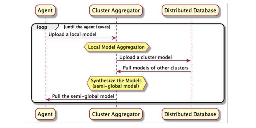
Figure 3.15 – The sequence of the semi-global model synthesis processes from uploading local models to pulling semi-global models
Let’s look at semi-global model synthesis using the flowchart between the agent, aggregator, and distributed database.
The aggregator receives a local model from an agent. When receiving the local model, the model filtering process will decide whether to accept the uploaded model or not. This framework can be implemented using many different methods, such as a basic scheme of checking the difference between the weights of the global and local models. If the model is not valid, just discard the local model.
Then, a cluster model is created by aggregating all the accepted local models. The aggregator stores the cluster model in a database, as well as simultaneously retrieving the cluster models generated by other cluster aggregators. A semi-global model is then synthesized from those cluster models and will be used in the agents that are assigned to the cluster aggregator.
Figure 3.16 shows how the cluster aggregator proceeds with cluster and semi-global model synthesis using a distributed database:

Figure 3.16 – The procedure and flow of semi-global model synthesis
An aggregator does not need to retrieve all the cluster models generated at each round to create a semi-global model. To synthesize a semi-global model, the global model can eventually converge based on the subset of models randomly selected by each aggregator. Using this approach, the robustness and independence of aggregators will be enhanced by compromising on the conditions to create the global model at every update. This framework can also resolve the bottlenecks in terms of computation and communication typical to centralized FL systems.
Summary
In this chapter, we discussed the potential architecture, procedure flow, and message sequences within an FL system. The typical FL system architecture consists of an aggregator, agents, and a database server. These three components are constantly communicating with each other to exchange system information and ML models to achieve model aggregation.
The key to implementing a good FL system is decoupling the critical components and carefully designing the interfaces between them. We focused on the aspect of the simplicity of its design so that further enhancement can be achieved by just adding additional components to the systems. Horizontal decentralized design can also help implement a scalable FL system.
In the following chapter, we will discuss the implementation details of achieving FL on the server side. As some critical aspects of the functionalities have been introduced in this chapter, you will be able to implement the basic system and smoothly run the simulation with some ML applications.
Further reading
Some of the concepts discussed in this chapter can be explored further by reading the following papers:
- Keith Bonawitz, Hubert Eichner, Wolfgang Grieskamp, Dzmitry Huba, Alex Ingerman, Vladimir Ivanov, Chloe Kiddon, et al. Towards Federated Learning at Scale: System Design. Proceedings of Machine Learning and Systems 1 (2019): 374–388, (https://arxiv.org/abs/1902.01046).
- Kairouz, P., McMahan, H. B., Avent, B., Bellet, A., Bennis, M., Bhagoji, A. N., and Zhao, S. (2021). Advances and Open Problems in Federated Learning. Foundations and Trends in Machine Learning, 14 (1 and 2): 1–210, (https://arxiv.org/abs/1912.04977).
- Stoica, I., Morris, R., Liben-Nowell, D., Karger, D., Kaashoek, M., Dabek, F., Balakrishnan, H. (2003). Chord: A Scalable Peer-to-Peer Lookup Protocol for Internet Applications, IEEE/ACM Transactions on Networking., Vol. 11, No. 1, pp 17–32, (https://resources.mpi-inf.mpg.de/d5/teaching/ws03_04/p2p-data/11-18-writeup1.pdf).
- Juan Benet. (2014). IPFS – Content Addressed, Versioned, P2P File System, (https://arxiv.org/abs/1407.3561).