6

Running the Federated Learning System and Analyzing the Results

In this chapter, you will run the federated learning (FL) system that has been discussed in previous chapters and analyze the system behaviors and the outcomes of the aggregated models. We will start by explaining the configuration of the FL system components in order to run the systems properly. Basically, after installing the simple FL system provided by our GitHub sample, you first need to pick up the server machines or instances to run the database and aggregator modules. Then, you can run agents to connect to the aggregator that is already running. The IP address of the aggregator needs to be correctly set up in each agent-side configuration. Also, there is a simulation mode so that you can run all the components on the same machine or laptop to just test the functionality of the FL system. After successfully running all the modules of the FL system, you will be able to see the data folder and a database created under the path that you set up in the database server as well as on the agent side. You will be able to check both the local and global models, trained and aggregated, so that you can download the recent or best-performing models from the data folders.

In addition, you can also see examples of running the FL system on a minimal engine and image classification. By reviewing the outcomes of the generated models and the performance data, you can understand the aggregation algorithms as well as the actual interaction of the models between an aggregator and agents.

In this chapter, we will cover the following main topics:

• Configuring and running the FL system
• Understanding what happens when the minimal example runs
• Running image classification and analyzing the results

Technical requirements

All the code files introduced in this chapter can be found on GitHub (https://github.com/tie-set/simple-fl).

Important note

You can use the code files for personal or educational purposes. Please note that we will not support deployments for commercial use and will not be responsible for any errors, issues, or damages caused by using the code.

Configuring and running the FL system

Configuring the FL system and installing its environment are simple enough to do. Follow the instructions in the next subsections.

Installing the FL environment

First, to run the FL system discussed in the previous chapter, clone the following repository to the machines that you want to run FL on using the following command:

git clone https://github.com/tie-set/simple-fl

Once done with the cloning process, change the directory to the simple-fl folder in the command line. The simulation run can be carried out using just one machine or using multiple systems. In order to run the FL process on one or multiple machines that include the FL server (aggregator), FL client (agent), and database server, you should create a conda virtual environment and activate it.

To create a conda environment in macOS, you will need to type the following command:

conda env create -n federatedenv -f ./setups/federatedenv.yaml

If you’re using a Linux machine, you can create the conda environment by using the following command:

conda env create -n federatedenv -f ./setups/federatedenv_linux.yaml

Then, activate the conda environment federatedenv when you run the code. For your information, the federatedenv.yaml and federatedenv_linux.yaml files can be found in the setups folder of the simple-fl GitHub repository and include the libraries that are used in the code examples throughout this book.

As noted in the README file of the GitHub repo, there are mainly three components to run: the database server, aggregator, and agent(s). If you want to conduct a simulation within one machine, you can just install a conda environment (federatedenv) on that machine.

If you want to create a distributed environment, you need to install the conda environment on all the machines you want to use, such as the database server on a cloud instance, the aggregator server on a cloud instance, and the local client machine.

Now that the installation process for the entire FL process is ready, let’s move on to configuring the FL system with configuration files.

Configuring the FL system with JSON files for each component

First, edit the configuration JSON files in the setups folder of the provided GitHub repository. These JSON files are read by a database server, aggregator, and agents to configure their initial setups. Again, the configuration details are explained as follows.

config_db.json

The config_db.json file deals with configuring a database server. Use the following information to properly operate the server:

• db_ip: The database server’s IP address (for example, localhost). If you want to run the database server on a cloud instance, such as an Amazon Web Services (AWS) EC2 instance, you can specify the private IP address of the instance.
• db_socket: The socket number used between the database and aggregator (for example, 9017).
• db_name: The name of the SQLite database (for example, sample_data).
• db_data_path: The path to the SQLite database (for example, ./db).
• db_model_path: The path to the directory to save all Machine Learning (ML) models (for example, ./db/models).

config_aggregator.json

The config_aggregator.json file deals with configuring an aggregator in the FL server. Use the following information to properly operate the aggregator:

• aggr_ip: The aggregator’s IP address (for example, localhost). If you want to run the aggregator server on a cloud instance, such as an AWS EC2 instance, you can specify the private IP address of the instance.
• db_ip: The database server’s IP address (for example, localhost). If you want to connect to the database server hosted on a different cloud instance, you can specify the public IP address of the database instance. If you host the database server on the same cloud instance as the aggregator’s instance, you can specify the same private IP address of the instance.
• reg_socket: The socket number used by agents to connect to an aggregator for the first time (for example, 8765).
• recv_socket: The socket number used to upload local models or poll to an aggregator from an agent. Agents will learn this socket information by communicating with an aggregator (for example, 7890).
• exch_socket: The socket number used to send global models back to an agent from an aggregator when a push method is used. Agents will learn this socket information by communicating with an aggregator (for example, 4321).
• db_socket: The socket number used between the database and an aggregator (for example, 9017).
• round_interval: The period of time after which an agent checks whether there are enough models to start an aggregation step (unit: seconds; for example, 5).
• aggregation_threshold: The percentage of collected local models required to start an aggregation step (for example, 0.85).
• polling: The flag to specify whether to use a polling method or not. If the flag is 1, use the polling method; if the flag is 0, use a push method. This value needs to be the same between the aggregator and agent.

config_agent.json

The config_agent.json file deals with configuring an agent in the FL client. Use the following information to properly operate the agent:

• aggr_ip: The aggregator server’s IP address (for example, localhost). If you want to connect to the aggregator server hosted on a cloud instance, such as an AWS EC2 instance, you can specify the public IP address of the aggregator instance.
• reg_socket: The socket number used by agents to join an aggregator for the first time (for example, 8765).
• model_path: The path to a local director in the agent machine to save local and global models and some state information (for example, ./data/agents).
• local_model_file_name: The filename to save local models in the agent machine (for example, lms.binaryfile).
• global_model_file_name: The filename to save local models in the agent machine (for example, gms.binaryfile).
• state_file_name: The filename to store the agent state in the agent machine (for example, state).
• init_weights_flag: 1 if the weights are initialized with certain values, 0 otherwise, where weights are initialized with zeros.
• polling: The flag to specify whether to use a polling method or not. If the flag is 1, use the polling method; if the flag is 0, use a push method. This value needs to be the same between the aggregator and agent.

Now, the FL systems can be configured using the configuration files explained in this section. Next, you will run the database and aggregator on the FL server side.

Running the database and aggregator on the FL server

In this section, you will configure the database and aggregator on the FL server side. Then, you will edit the configuration files in the setups folder of the simple-fl GitHub repo. After that, you will run pseudo_db first, and then server_th, as follows:

python -m fl_main.pseudodb.pseudo_db

python -m fl_main.aggregator.server_th

Important note

If the database server and aggregator server are running on different machines, you will need to specify the IP address of the database server or instance of the aggregator. The IP address of the database server can be modified in the config_aggregator.json file in the setups folder. Also, if both the database and aggregator instances are running in public cloud environments, the IP address of the configuration files of those servers needs to be the private IP address. Agents need to connect to the aggregator using the public IP address and the connecting socket (port number) needs to be open to accept inbound messages.

After you start the database and aggregator servers, you will see a message such as the following in the console:

# Database-side Console Example
INFO:root:--- Pseudo DB Started ---

On the aggregator side of the console, you will see something like the following:

# Aggregator-side Console Example
INFO:root:--- Aggregator Started ---

Behind this aggregator server, the model synthesis module is running every 5 seconds, where it starts checking whether the number of collected local models is more than the number that the aggregation threshold defines.

We have now run the database and aggregator modules and are ready to run a minimal example with the FL client.

Running a minimal example with the FL client

In the previous chapter, we talked about the integration of local ML engines into the FL system. Here, using a minimal sample that does not have actual training data, we will try to run the FL systems that have been discussed. This minimal example can be used as a template when implementing any locally distributed ML engine.

Before running the minimal example, you should check whether the database and aggregator servers are running already. Then, run the following command:

python -m examples.minimal.minimal_MLEngine

In this case, only one agent with a minimal ML engine is connected. Thus, the aggregation happens every time this default agent uploads the local model.

Note that if the aggregator server is running on a different machine, you will need to specify the public IP address of the aggregator server or instance. The IP address of the aggregator can be modified in the config_agent.json file in the setups folder. We also recommend setting the polling flag to 1 when running the aggregator and database in a cloud instance.

Figure 6.1 shows an example of the console screen when running a database server:

Figure 6.1 – Example of a database-side console

Figure 6.2 shows an example of the console screen when running an aggregator:

Figure 6.2 – Example of an aggregator-side console

Figure 6.3 shows an example of the console screen when running an agent:

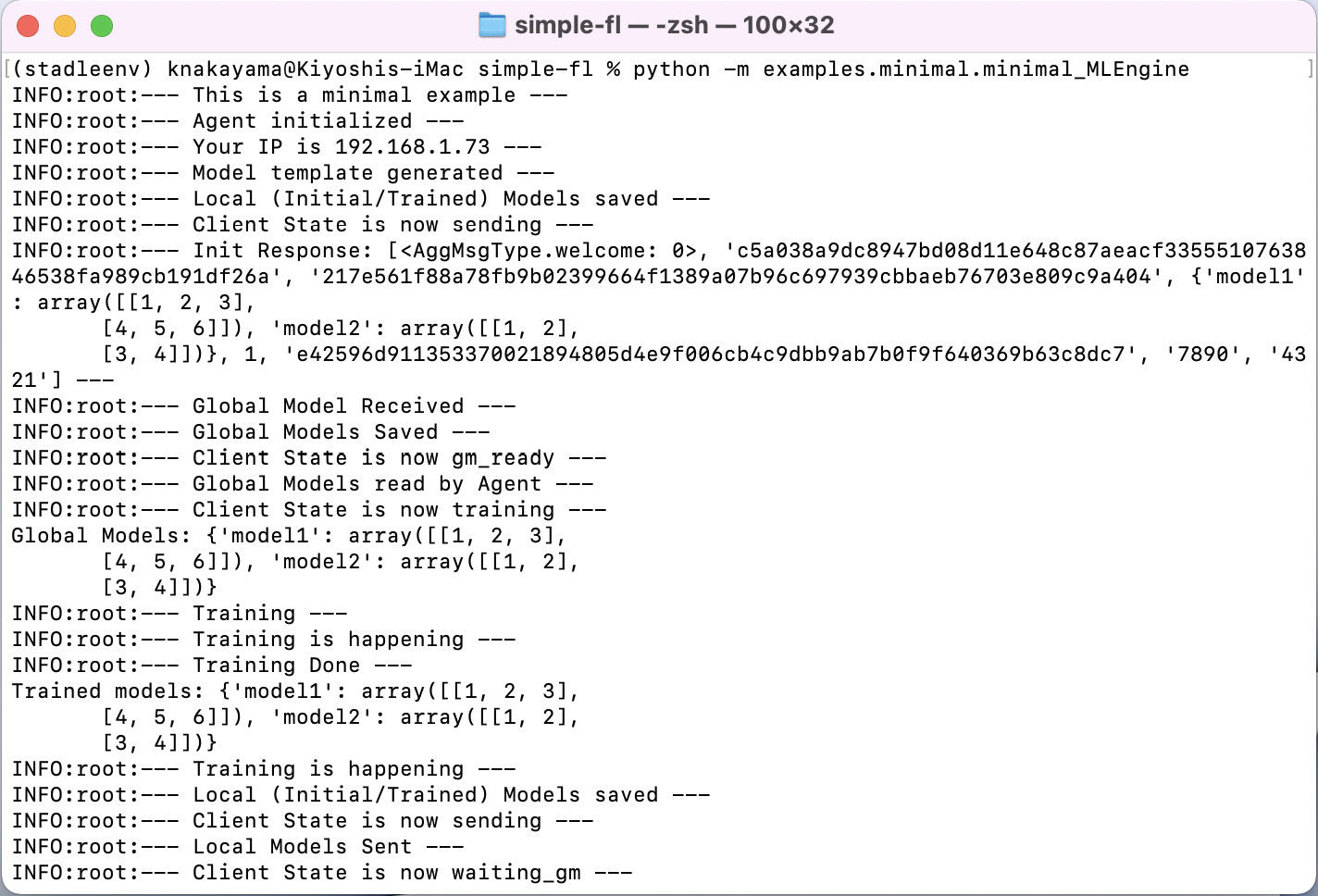
Figure 6.3 – Example of an agent-side console

Now we know how to run all the FL components: a database, aggregator, and agent. In the next section, we will examine how outputs are generated by running the FL system.

Data and database folders

After running the FL system, you will notice that the database folder and data folder are created under the locations that you specified in the config files of the database and agent.

For example, the db folder is created under db_data_path, written in the config_db.json file. In the database folder, you will find the SQLite database, such as model_data12345.db, where the metadata of local and cluster global models is stored, as well as a models folder that contains all the actual local models uploaded by the agents and global models created by the aggregator.

Figure 6.4 shows the SQLite database and ML model files in a binary file format stored in the db folder created by running the minimal example code:

Figure 6.4 – The SQLite database and ML model files in a binary file format stored in the db folder

The data folder is created under an agent device at the location of the model_path, a string value defined in config_agent.json. In the example run of the minimal example, the following files are created under the data/agents/default-agent folder:

• lms.binaryfile: A binary file containing a local model created by the agent
• gms.binaryfile: A binary file containing a global model created by the aggregator sent back to the agent
• state: A file that has an integer value that indicates the state of the client itself

Figure 6.5 shows the structure of the agent-side data, which includes global and local ML models represented with a binary file format, as well as the file reflecting the FL client state:

Figure 6.5 – Data of the agents including global and local ML models with a binary file format as well as the client state

Now we understand where the key data, such as global and local models, is stored. Next, we will take a closer look at the database using SQLite.

Databases with SQLite

The database created in the db folder can be viewed using any tool to show the SQLite database that can open files with the ***.db format. The database tables are defined in the following sections.

Local models in a database

Figure 6.6 shows sample database entries related to uploaded local models where each entry lists the local model ID, the time that the model was generated, the ID of the agent that uploaded the local model, round information, performance metrics, and the number of data samples:

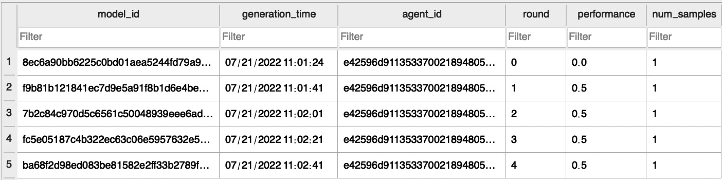
Figure 6.6 – Sample database entries related to uploaded local models

Cluster models in a database

Figure 6.7 shows sample database entries related to uploaded cluster models where each entry lists the cluster model ID, the time that the model was created, the ID of the aggregator that created this cluster model, round information, and the number of data samples:

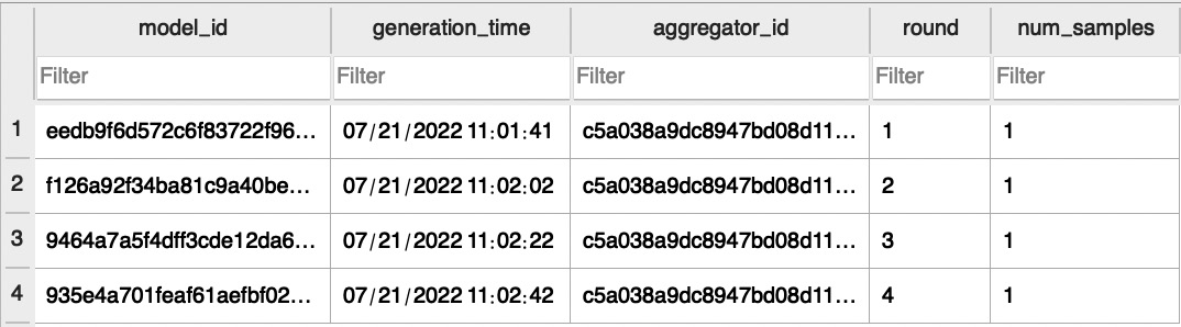
Figure 6.7 – Sample database entries related to uploaded cluster models

Now we have learned how to configure and run the FL system with a minimal example and how to examine the results. In the next section, you will learn about the behavior of the FL system and what happens when the minimal example is run.

Understanding what happens when the minimal example runs

Understanding the behavior of the entire FL system step by step will help you design applications with FL enabled and further enhance the FL system itself. Let us first look into what happens when we run just one agent by printing some procedures of the agent and aggregator modules.

Running just one minimal agent

Let’s run the minimal agent after running the database and aggregator servers and see what happens. When the agent is started with the minimal ML engine, you will see the following messages in the agent console:

# Agent-side Console Example
INFO:root:--- This is a minimal example ---
INFO:root:--- Agent initialized —
INFO:root:--- Your IP is xxx.xxx.1.101 ---

When the agent initializes the model to be used for FL, it shows this message, and if you look at the state file, it has entered the sending state, which will trigger sending models to the aggregator when the FL client is started:

# Agent-side Console Example
INFO:root:--- Model template generated ---
INFO:root:--- Local (Initial/Trained) Models saved ---
INFO:root:--- Client State is now sending ---

Then, after the client is started with the start_fl_client function, the participation message is sent to the aggregator. Here is the participation message sent to the aggregator:

[
        <AgentMsgType.participate: 0>, # Agent Message Type
        'A89fd1c2d9*****', # Agent ID
        '047b18ddac*****',    # Model ID
        {
                'model1': array([[1, 2, 3], [4, 5, 6]]), 
                'model2': array([[1, 2], [3, 4]])
        }, # ML Models
        True,    # Init weights flag
        False, # Simulation flag
        0, # Exch Port
        1645141807.846751, # Generated Time of the models
        {'accuracy': 0.0, 'num_samples': 1}, # Meta information 
        'xxx.xxx.1.101' # Agent's IP Address
]

The participation message to the aggregator includes the message type, agent ID, model ID, ML model with NumPy, initialization weights flag, simulation flag, exchange port number, time the models were generated, and meta information such as performance metrics and the agent’s IP address.

The agent receives the welcome message from an aggregator confirming the connection of this agent, which also includes the following information:

# Agent-side Console Example
INFO:root:--- Init Response: [
        <AggMsgType.welcome: 0>, # Message Type
        '4e2da*****', # Aggregator ID
        '23487*****', # Model ID 
        {'model1': array([[1, 2, 3], [4, 5, 6]]), 
         'model2': array([[1, 2], [3, 4]])}, # Global Models
        1, # FL Round
        'A89fd1c2d9*****', # Agent ID
        '7890', # exch_socket number
        '4321' # recv_socket number
] ---

On the aggregator side, after this agent sends a participation message to the aggregator, the aggregator confirms the participation and pushes this initial model to the database:

# Aggregator-side Console Example
INFO:root:--- Participate Message Received ---
INFO:root:--- Model Formats initialized, model names: ['model1', 'model2'] ---
INFO:root:--- Models pushed to DB: Response ['confirmation'] ---
INFO:root:---  Global Models Sent to A89fd1c2d9***** ---
INFO:root:--- Aggregation Threshold (Number of agents needed for aggregation): 1 ---
INFO:root:--- Number of collected local models: 0 ---
INFO:root:--- Waiting for more local models to be collected ---

In the database server-side console, you can also check that the local model is sent from the aggregator and the model is saved in the database:

# DB-side Console Example
INFO:root:Request Arrived
INFO:root:--- Model pushed: ModelType.local ---
INFO:root:--- Local Models are saved ---

After the aggregator sends the global model back to the agent, the agent receives and saves it and changes the client state from waiting_gm to gm_ready, indicating the global model is ready for retraining locally:

# Agent-side Console Example
INFO:root:--- Global Model Received ---
INFO:root:--- Global Models Saved ---
INFO:root:--- Client State is now gm_ready ---

Here is the message sent to the agent from an aggregator, including the global model. The contents of the message include the message type, aggregator ID, cluster model ID, FL round, and ML models with NumPy:

[
        <AggMsgType.sending_gm_models: 1>, # Message Type
        '8c6c946472*****', # Aggregator ID
        'ab633380f6*****', # Global Model ID
        1, # FL Round Info 
        {     
                'model1': array([[1., 2., 3.],[4., 5., 6.]]), 
                'model2': array([[1., 2.],[3., 4.]])
        } # ML models
]

Then, the agent reads the global models to proceed with using them for local training and changes the client state to training:

# Agent-side Console Example
INFO:root:--- Global Models read by Agent ---
INFO:root:--- Client State is now training ---
INFO:root:--- Training ---
INFO:root:--- Training is happening ---
INFO:root:--- Training is happening ---
INFO:root:--- Training Done ---
INFO:root:--- Local (Initial/Trained) Models saved ---
INFO:root:--- Client State is now sending ---
INFO:root:--- Local Models Sent ---
INFO:root:--- Client State is now waiting_gm ---
INFO:root:--- Polling to see if there is any update (shown only when polling) ---
INFO:root:--- Global Model Received ---
INFO:root:--- The global models saved ---

After the preceding local training process, the agent proceeds with sending the trained local models to the aggregator and changes the client state to waiting_gm, which means it waits for the global model with the polling mechanism.

Here is the message sent to the aggregator as a trained local model message. The contents of the message include message type, agent ID, model ID, ML models, generated time of the models, and metadata such as performance data:

[
        <AgentMsgType.update: 1>, # Agent's Message Type
        'a1031a737f*****', # Agent ID
        'e89ccc5dc9*****', # Model ID
        {
                'model1': array([[1, 2, 3],[4, 5, 6]]), 
                'model2': array([[1, 2],[3, 4]])
        }, # ML Models
            1645142806.761495, # Generated Time of the models
        {'accuracy': 0.5, 'num_samples': 1} # Meta information
]

Then, in the aggregator, after the local model is pushed to the database, it shows the change in the buffer, that the number of collected local models is up to 1 from 0, thus indicating that enough local models are collected to start the aggregation:

# Aggregator-side Console Example
INFO:root:--- Models pushed to DB: Response ['confirmation'] ---
INFO:root:--- Local Model Received ---
INFO:root:--- Aggregation Threshold (Number of agents needed for aggregation): 1 ---
INFO:root:--- Number of collected local models: 1 ---
INFO:root:--- Enough local models are collected. Aggregation will start. ---

Then, aggregation for round 1 happens and the cluster global models are formed, pushed to the database, and sent to the agent once the polling message arrives from the agent. The aggregator can also push the message back to the agent via a push method:

# Aggregator-side Console Example
INFO:root:Round 1
INFO:root:Current agents: [{'agent_name': 'default_agent', 'agent_id': 'A89fd1c2d9*****', 'agent_ip': 'xxx.xxx.1.101', 'socket': 7890}]
INFO:root:--- Cluster models are formed ---
INFO:root:--- Models pushed to DB: Response ['confirmation'] ---
INFO:root:--- Global Models Sent to A89fd1c2d9***** ---

On the database server side, the cluster global model is received and pushed to the database:

# DB-side Console Example
INFO:root:Request Arrived
INFO:root:--- Model pushed: ModelType.cluster ---
INFO:root:--- Cluster Models are saved ---

This process in this section is repeated after cluster models are generated and saved for the upcoming FL round and the round of FL proceeds with this interaction mechanism.

If you look at both the local and cluster global models, they are as follows:

{
        'model1': array([[1, 2, 3],[4, 5, 6]]), 
        'model2': array([[1, 2],[3, 4]])
}

This means only one fixed model is used all the time even if aggregation happens, so the global model is exactly the same as the initial one as the dummy training process is used here.

We will now look into the results when running two minimal agents in the next section.

Running two minimal agents

With the database and aggregator servers running, you can run many agents using the minimal_MLEngine.py file in the simple-fl/examples/minimal folder.

You should run the two individual agents from different local machines by specifying the IP address of the aggregator to connect those agents with the minimal ML example.

You can also run multiple agents from the same machine for simulation purposes by specifying the different port numbers for the individual agents.

In the code provided in the simple-fl repository on GitHub, you can run the multiple agents by using the following command:

python -m examples.minimal.minimal_MLEngine [simulation_flag] [gm_recv_port] [agent_name]

To conduct the simulation, simulation_flag should be set to 1. gm_recv_port is the port number to receive the global models from the aggregator. The agent will be notified of the port number by the aggregator through the response of a participation message. Also, agent_name is the name of the local agent and the directory name storing the state and model files. This needs to be unique for every agent.

For instance, you can run the first and second agents with the following commands:

# First agent

python -m examples.minimal.minimal_MLEngine 1 50001 a1

# Second agent

python -m examples.minimal.minimal_MLEngine 1 50002 a2

You can edit the configuration JSON files in the setups folder if needed. In this case, agg_threshold is set to 1.

When you run the simulation in the database server running a minimal example with multiple agents, the console screen will look similar to that in Figure 6.1.

Figure 6.8 shows the console screen of a simulation in the aggregator server running a minimal example using dummy ML models:

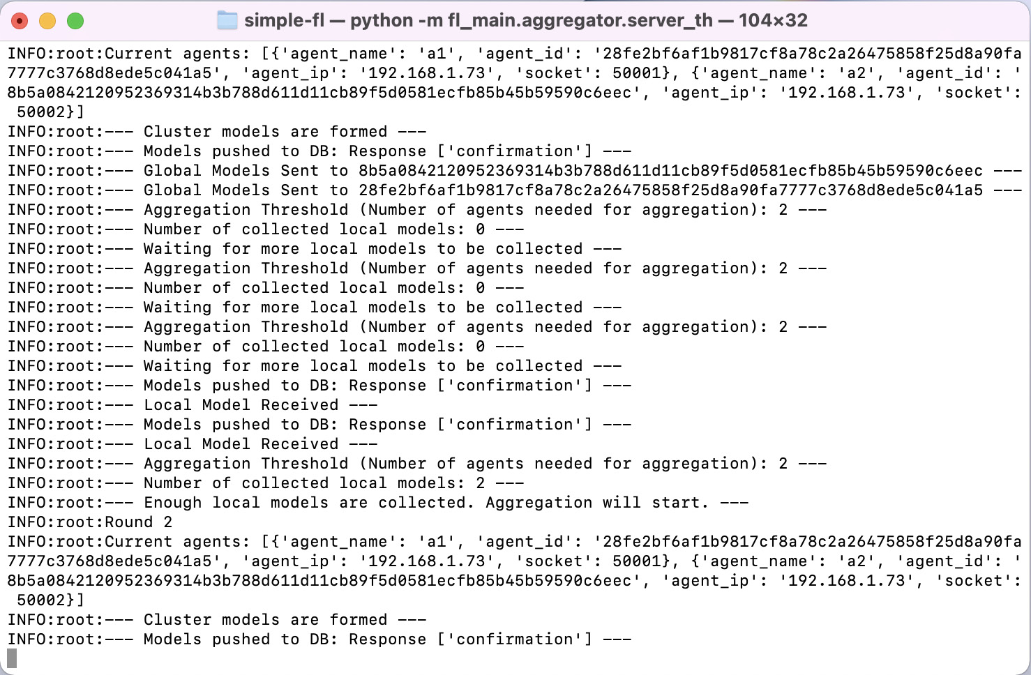
Figure 6.8 – Example of an aggregator-side console running a minimal example connecting two agents

Figure 6.9 shows the console screen of a simulation in one of the agents running a minimal example using dummy ML models:

Figure 6.9 – Example of agent 1’s console running a minimal example using dummy ML models

Figure 6.10 shows the console screen of a simulation in another agent running a minimal example using dummy ML models:

Figure 6.10 – Example of agent 2’s console running a minimal example using dummy ML models

Now we know how to run the minimal example with two agents. In order to further look into the FL procedure using this example, we will answer the following questions:

• Has aggregation been done correctly for the simple cases?
• Has the FedAvg algorithm been applied correctly?
• Does aggregation threshold work with connected agents?

After running and connecting the two agents, the aggregator will wait to receive two models from the two connected agents, as follows:

# Aggregator-side Console Example
INFO:root:--- Aggregation Threshold (Number of agents needed for aggregation): 2 ---
INFO:root:--- Number of collected local models: 0 ---
INFO:root:--- Waiting for more local models to be collected ---

In this case, the aggregation threshold is set to 1.0 in the config_aggregator.json file in the setups folder, so the aggregator needs to collect all the models from connected agents, meaning it needs to receive local ML models from all the agents that are connected to the aggregator.

Then, it receives one model from one of the agents and the number of collected local models is increased to 1. However, as the aggregator is still missing one local model, it does not start aggregation yet:

# Aggregator-side Console Example
INFO:root:--- Local Model Received ---
INFO:root:--- Aggregation Threshold (Number of agents needed for aggregation): 2 ---
INFO:root:--- Number of collected local models: 1 ---
INFO:root:--- Waiting for more local models to be collected ---

On the agent side, after the local models are sent to the aggregator, it will wait until the cluster global model to be created in the aggregator and sent back to the agent. In this way, you can synchronize the FL process at the agent side and automate the local training procedure when the global model is sent back to the agent and ready for retraining.

After the aggregator receives another local model, enough models are collected to start the aggregation process:

# Aggregator-side Console Example
INFO:root:--- Local Model Received ---
INFO:root:--- Aggregation Threshold (Number of agents needed for aggregation): 2 ---
INFO:root:--- Number of collected local models: 2 ---
INFO:root:--- Enough local models are collected. Aggregation will start. ---

It will finally start the aggregation for the first round, as follows:

# Aggregator-side Console Example
INFO:root:Round 1
INFO:root:Current agents: [{'agent_name': 'a1', 'agent_id': '1f503*****', 'agent_ip': 'xxx.xxx.1.101', 'socket': 50001}, {'agent_name': 'a2', 'agent_id': '70de8*****', 'agent_ip': 'xxx.xxx.1.101', 'socket': 50002}]
INFO:root:--- Cluster models are formed ---
INFO:root:--- Models pushed to DB: Response ['confirmation'] ---
INFO:root:--- Global Models Sent to 1f503***** ---
INFO:root:--- Global Models Sent to 70de8***** ---

Here, let’s look at the agent-side ML models that are locally trained:

# Agent 1's Console Example
INFO:root:--- Training ---
INFO:root:--- Training is happening ---
INFO:root:--- Training Done ---
Trained models: {'model1': array([[1, 2, 3],
             [4, 5, 6]]), 'model2': array([[1, 2],
             [3, 4]])}
INFO:root:--- Local (Initial/Trained) Models saved ---

Also, let’s look at another agent’s ML models that are locally trained:

# Agent 2's Console Example
INFO:root:--- Training ---
INFO:root:--- Training is happening ---
INFO:root:--- Training Done ---
Trained models: {'model1': array([[3, 4, 5],
             [6, 7, 8]]), 'model2': array([[3, 4],
             [5, 6]])}
INFO:root:--- Local (Initial/Trained) Models saved ---

As in the models sent to the aggregator from agents 1 and 2, if FedAvg is correctly applied, the global model should be the averaged value of these two models. In this case, the number of data samples is the same for both agents 1 and 2, so the global model should just be an average of the two models.

So, let’s look at the global models that are generated in the aggregator:

# Agent 1 and 2's Console Example
Global Models: {'model1': array([[2., 3., 4.],
             [5., 6., 7.]]), 'model2': array([[2., 3.],
             [4., 5.]])}

The received model is the average of the two local models and thus averaging has been correctly conducted.

The database and data folders are created in the model_path specified in the agent configuration file. You can look at the database values with an SQLite viewer application and look for some models based on the model ID.

Now that we understand what’s happening with minimal example runs, in the next section, we will run a real ML application using an image classification model using a Convolutional Neural Network (CNN).

Running image classification and analyzing the results

This example demonstrates the use of this FL framework for image classification tasks. We will use a famous image dataset, CIFAR-10 (URL: https://www.cs.toronto.edu/~kriz/cifar.html), to show how an ML model grows through the FL process over time. However, this example is only given for the purposes of using the FL system we have discussed so far and is not focused on maximizing the performance of the image classification task.

Preparing the CIFAR-10 dataset

The following is the information required related to the dataset size, the training and test data, the number of classes, and the image size:

• Dataset size: 60,000 images
• Training data: 50,000 images
• Test data: 10,000 images
• Number of classes: 10 (airplane, automobile, bird, cat, deer, dog, frog, horse, ship, and truck)
• Each class has 6,000 images
• Image size: 32x32 pixels, in color

Figure 6.11 shows a collection of sample pictures of 10 different classes in the dataset with 10 random images for each:

Figure 6.11 – The classes in the dataset as well as 10 random images for each category (the images are adapted from https://www.cs.toronto.edu/~kriz/cifar.html)

Now that the dataset is prepared, we will look into a CNN model used for the FL process.

The ML model used for FL with image classification

Here is the description of the ML model architecture of the CNN model used in this image classification example. To learn more about what the CNN is, you can find many useful study resources, such as https://cs231n.github.io/convolutional-networks/:

• Conv2D
• MaxPool2D (maximum pooling)
• Conv2D
• 3 fully-connected layers

The script to define the CNN model is already designed and can be found in cnn.py in examples/image_classification in the simple-fl repository on GitHub. Next, we will run the image classification application with the FL system.

How to run the image classification example with CNN

As mentioned in the installation steps at the beginning of this chapter, we first install the necessary libraries with federatedenv, and then install torch and torchvision after that:

pip install torch

pip install torchvision

You can configure many settings through the JSON config files in the setups folder of the simple-fl repo of GitHub. For more details, you can read the general description of the config files in our setups documentation (https://github.com/tie-set/simple-fl/tree/master/setups).

First, you can run two agents. You can increase the number of agents running on the same device by specifying the appropriate port numbers.

As you already know, the first thing you can do is run the database and aggregator:

# FL server side
python -m fl_main.pseudodb.pseudo_db
python -m fl_main.aggregator.server_th

Then, start the first and second agents to run the image classification example:

# First agent
python -m examples.image_classification.classification
_engine 1 50001 a1
# Second agent
python -m examples.image_classification.classification
_engine 1 50002 a2

To simulate the actual FL scenarios, the amount of training data accessible from each agent can be limited to a specific number. This should be specified with the num_training_data variable in classification_engine.py. By default, it uses 8,000 images (2,000 batches) for each round.

Now that we can run the two agents to test the FL process using CNN models, let us look further into the results by running the image classification example.

Evaluation of running the image classification with CNN

The performance data (the accuracy of each local model cluster model) is stored in our database. You can access the corresponding .db file to see the performance history.

The DataManager instance (defined in ic_training.py) has a function to return one batch of images and their labels (get_random_images). You can use this function to show the actual labels and the predicted labels by the trained CNN on specific images.

Figure 6.12 shows a plot of the learning performance from our experimental runs on our side; the results may look different when you run it with your own settings:

Figure 6.12 – Plot of the learning performance from the experimental runs for FL using CNN for image classification

Again, as we only use two agents here, the results just look slightly different. However, with the proper hyperparameter settings, data amount, and the number of agents, you will be able to carry out an FL evaluation that produces meaningful results, which we would like you to explore on your own, as the focus here is just how to connect the actual ML models to this FL environment.

Running five agents

You can easily run five agents for the image classification application by just specifying different port numbers and agent names in the terminal. The results look similar to what we discussed in the previous section except the real ML models are connected (in this case, the ML model being aggregated is CNN). After running the five agents, the data and database folders look like in Figure 6.13:

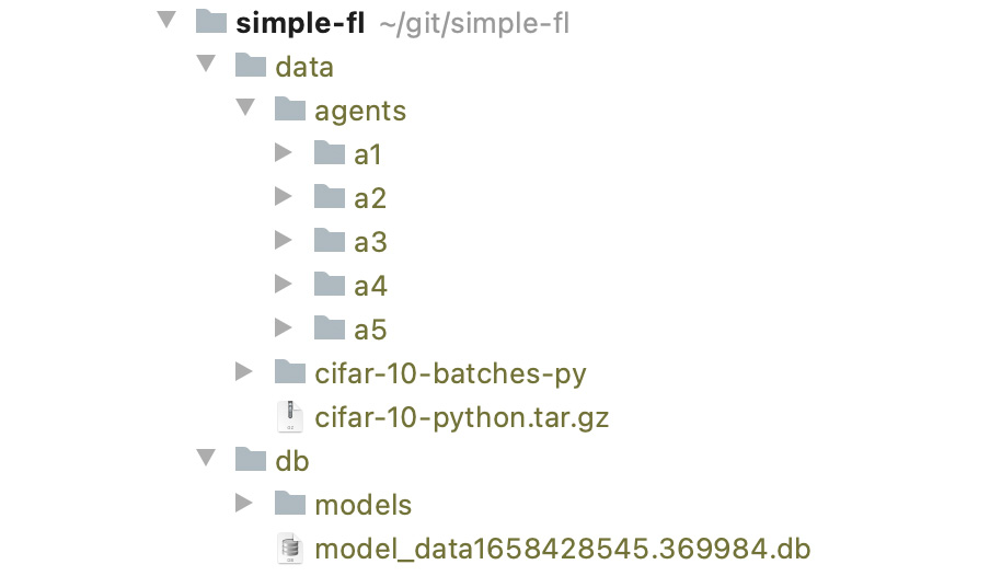
Figure 6.13 – Results to be stored in each folder with the agent’s unique name

Figure 6.14 shows the uploaded local models in the database with information about the local model ID, the time the models were generated, the ID of the agent that uploaded the local model, performance metrics, and round information:

Figure 6.14 – Information about the local models in the database 

If you look at the database in Figure 6.14, there are five models collected by the five agents with local performance data.

For each round, those five local models are aggregated to produce a cluster global model, as in the cluster_models table in the database, as shown in Figure 6.15. The database storing cluster models has information about the cluster model ID, the time the models were generated, the ID of the aggregator that created the cluster model, and round information:

Figure 6.15 – Information about the cluster models in the database

In this way, you can connect as many agents as possible. It is up to you to optimize the settings of the local ML algorithms to obtain the best-performing federated models out of the FL system.

Summary

In this chapter, we discussed the execution of FL systems in detail and how the system will behave according to the interactions between the aggregator and agents. The step-by-step explanation of the FL system behavior based on the outcomes of the console examples guides you to understand the aggregation process of the FedAvg algorithm. Furthermore, the image classification example showed how CNN models are connected to the FL system and how the FL process increases the accuracy through aggregation, although this was not optimized to maximize the training results but simplified to validate the integration using CNN.

With what you have learned in this chapter, you will be able to design your own FL applications integrating the principles and framework introduced in this book, and furthermore, will be able to assess the FL behavior on your own to see whether the whole flow of the FL process and model aggregation is happening correctly and consistently.

In the next chapter, we will cover a variety of model aggregation methods and show how FL works well with those aggregation algorithms.