A for loop with a large number of iterations is a good candidate for parallel execution, and Julia has a special construct to do this: the @parallel macro, which can be used for the for loops and comprehensions.

Let's calculate an approximation for Π using the famous Buffon's needle problem. If we drop a needle onto a floor with equal parallel strips of wood, what is the probability that the needle will cross a line between two strips? Let's take a look at the following screenshot:

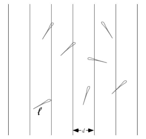
Without getting into the mathematical intricacies of this problem (if you are interested, see http://en.wikipedia.org/wiki/Buffon's_needle), a buffon(n) function can be deduced from the model assumptions that returns an approximation for Π when throwing the needle n times (assuming the length of the needle, l, and the width, d, between the strips both equal 1):

// code in Chapter 8parallel_loops_maps.jl
function buffon(n)
  hit = 0
  for i = 1:n
    mp = rand()
    phi = (rand() * pi) - pi / 2 # angle at which needle falls
    xright = mp + cos(phi)/2 # x location of needle
    xleft = mp - cos(phi)/2
    # does needle cross either x == 0 or x == 1?
    p = (xright >= 1 || xleft <= 0) ? 1 : 0
    hit += p
  end
  miss = n - hit
  piapprox = n / hit * 2
end

With ever-increasing n, the calculation time increases, because the number of the for iterations that have to be executed in one thread on one processor increases, but we also get a better estimate for Π:

@time buffon(100000)
   0.208500 seconds (504.79 k allocations: 25.730 MiB, 7.10% gc time)
 3.1441597233139444 

@time buffon(100000000)
  4.112683 seconds (5 allocations: 176 bytes)
   3.141258861373451 

However, what if we could spread the calculations over the available processors? For this, we have to rearrange our code a bit. In the sequential version, the variable hit is increased on every iteration inside the for loop with the p amount (which is 0 or 1). In the parallel version, we rewrite the code, so that this p is exactly the result of the for loop (one calculation) done on one of the involved processors.

Julia also provides a @distributed macro that acts on a for loop, splitting the range and distributing it to each process. It optionally takes a "reducer" as its first argument. If a reducer is specified, the results from each remote procedure will be aggregated using the reducer. In the following example, we use the (+) function as a reducer, which means that the last values of the parallel blocks on each worker will be summed to calculate the final value of hit:

function buffon_par(n)
  hit = @distributed (+) for i = 1:n
      mp = rand()
      phi = (rand() * pi) - pi / 2
      xright = mp + cos(phi)/2
      xleft = mp - cos(phi)/2
       (xright >= 1 || xleft <= 0) ? 1 : 0
    end
  miss = n - hit
  piapprox = n / hit * 2
end

On my machine with eight processors, this gives the following results:

@time buffon_par(100000)
  1.058487 seconds (951.35 k allocations: 48.192 MiB, 2.04% gc time)
 3.15059861373661 

@time buffon_par(100000000)
  0.735853 seconds (1.84 k allocations: 133.156 KiB)
 3.1418106012575633

We see much better performance for the higher number of iterations (a factor of 5.6 in this case). By changing a normal for loop into a parallel-reducing version, we were able to get substantial improvements in the calculation time, at the cost of higher memory consumption. In general, always test whether the parallel version really is an improvement over the sequential version in your specific case!

The first argument of @distributed is the reducing operator (here, (+)), the second is the for loop, which must start on the same line. The calculations in the loop must be independent of one another, because the order in which they run is arbitrary, given that they are scheduled over the different workers. The actual reduction (summing up in this case) is done on the calling process.

Any variables used inside the parallel loop will be copied (broadcasted) to each process. Because of this, the code, such as the following, will fail to initialize the arr array, because each process has a copy of it:

arr = zeros(100000)
@distributed for i=1:100000
  arr[i] = i
end

Afterward the loop, arr still contains all the zeros, because it is the copy on the master worker.

If the computational task is to apply a function to all elements in some collection, you can use a parallel map operation through the pmap function. The pmap function takes the following form: pmap(f, coll), applies an f function on each element of the coll collection in parallel, but preserves the order of the collection in the result. Suppose we have to calculate the rank of a number of large matrices. We can do this sequentially, as follows:

using LinearAlgebra
function rank_marray()
  marr = [rand(1000,1000) for i=1:10]
  for arr in marr
      println(LinearAlgebra.rank(arr))
  end
end

@time rank_marray() # prints out ten times 1000
7.310404 seconds (91.33 k allocations: 162.878 MiB, 1.15% gc time)

In the following, parallelizing also gives benefits (a factor of 1.6):

function prank_marray()
  marr = [rand(1000,1000) for i=1:10]
  println(pmap(LinearAlgebra.rank, marr))
end

@time prank_marray()
5.966216 seconds (4.15 M allocations: 285.610 MiB, 2.15% gc time)

The @distributed macro and pmap are both powerful tools to tackle map-reduce problems.

Julia's model for building a large parallel application works by means of a global distributed address space. This means that you can hold a reference to an object that lives on another machine participating in a computation. These references are easily manipulated and passed around between machines, making it simple to keep track of what's being computed where. Also, machines can be added in mid-computation when needed.