Chapter 1. Building applications for the intelligent web
This chapter covers
- Recognizing intelligence on the web
- Types of intelligent algorithms
- Evaluating intelligent algorithms
The intelligent web means different things to different people. To some it represents the evolution of the web into a more responsive and useful entity that can learn from and react to its users. To others it represents the inclusion of the web into many more aspects of our lives. To me, far from being the first iteration of Skynet, in which computers take over in a dystopian future, the intelligent web is about designing and implementing more naturally responsive applications that make our online experiences better in some quantifiable way. There’s a good chance that every reader has encountered machine intelligence on many separate occasions, and this chapter will highlight some examples so that you’ll be better equipped to recognize these in the future. This will, in turn, help you understand what’s really happening under the hood when you interact with intelligent applications again.
Now that you know this book isn’t about writing entities that will try to take over the world, we should perhaps discuss some other things that you won’t find within these pages! First, this is very much a back-end book. In these pages, you won’t learn about beautiful interactive visualizations or platforms. For this, we refer you to excellent publications by Scott Murray,[1] David McCandless,[2] and Edward Tufte.[3] Suffice to say that we don’t have space here to do this topic justice along with what we’re about to cover. Also, this book won’t teach you statistics; but to gain the most from the book we’ll assume you have a 101 level of knowledge or higher, in that you should have at least taken a course in statistics at some point in the past.
Scott Murray, Interactive Data Visualization for the Web (O’Reilly, 2013).
David McCandless, Information Is Beautiful (HarperCollins, 2010).
Edward Tufte, The Visual Display of Quantitative Information (Graphics Press USA, 2001).
This is also not a book about data science. A plethora of titles are available that will help the data science practitioner, and we do hope that this book will be useful to data scientists, but these chapters contain little detail about how to be a data scientist. For these topics we refer you to the texts by Joel Grus[4] and Foster Provost and Tom Fawcett.[5]
Joel Grus, Data Science From Scratch: First Principles with Python (O’Reilly, 2015).
Foster Provost and Tom Fawcett, Data Science for Business (O’Reilly Media, 2013).
Nor is this a detailed book about algorithm design. We’ll often skim over details as to the design of algorithms and provide more intuition than a deep dive into specifics. This will allow us to cover much more ground, perhaps at the cost of some rigor. Think of each chapter as a trail of breadcrumbs leading you through the important aspects of that approach and nudging you toward resources where you can learn more.
Although many of the examples within the pages of this book are written using scikit-learn (http://scikit-learn.org), this isn’t a book about scikit-learn! That is merely the tool by which we can demonstrate the approaches presented in this book. We’ll never provide an example without at least an intuitive introduction as to why the algorithm works. In some cases we’ll go deeper, but in many cases you should continue your research outside this book.
So what, then, is this book about? We’ll cover the tools that provide an end-to-end view of intelligent algorithms as we see them today. We’ll talk about the information that’s collected about you, the average web user, and how that information can be channeled into useful streams so that it can be used to make predictions about your behavior—changing those predictions as your behavior changes. This means we’ll often deviate from the standard “algorithm 101” book, in favor of giving you a flavor (!) of all the important aspects of intelligent algorithms.
We’ll even discuss (in the appendix) a publish/subscribe technology that allows large quantities of data to be organized during ingestion. Although this has no place in a book that’s strictly about data science or algorithms, we believe that it has a fundamental place in a book about the intelligent web. This doesn’t mean we ignore data science or algorithms—quite the contrary! We’ll cover most of the important algorithms used by the majority of the leading players in the intelligent-algorithm space. Where possible, we reference known examples of these in the wild, so that you can test your knowledge against the behavior of such systems—and no doubt impress your friends!
But we’re getting ahead of ourselves. In this chapter, we’ll provide several examples of the application of intelligent algorithms that you should find immediately recognizable. We’ll talk more about what intelligent algorithms can’t do, before providing you with a taxonomy of the field that can be used to hang your newly learned concepts on. Finally, we’ll present you with a number of methods to evaluate intelligent algorithms and impart to you some useful things to know.
We already hear you asking, “What is an intelligent algorithm?” For the purposes of this book, we’ll refer to any algorithm that uses data to modify its behavior as intelligent. Remember that when you interact with an algorithm, you’re merely interacting with a set of distinct rules. Intelligent algorithms differ in that they can change their behavior as they run, often resulting in a user experience that many would say is intelligent. Figure 1.1 summarizes this behavior. Here you see an intelligent algorithm responding to events within the environment and making decisions. By ingesting data from the context in which it operates (which may include the event itself), the algorithm is evolving. It evolves in the sense that the decision is no longer deterministic given the event. The intelligent algorithm may make different decisions at different points, depending on the data it has ingested.
Figure 1.1. Overview of an intelligent algorithm. Such algorithms display intelligence because the decisions they make change depending on the data they’ve received.

1.1. An intelligent algorithm in action: Google Now
To demonstrate this concept, we’ll try to deconstruct the operation of Google Now. Note that the specific details of this project are proprietary to Google, so we’ll be relying on our own experience to illustrate how this system might work internally.
For those of you with Android devices, this product may be immediately recognizable, but for the iOS users among us, Google Now is Google’s answer to Siri and has the product tagline “The right information at just the right time.” This is essentially an application that can use various sources of information and alert you about nearby restaurants, events, traffic jams, and the like that it believes will be of interest to you. To demonstrate the concept of an intelligent algorithm, let’s take an even more concrete example from Google Now. When it detects a traffic jam on your normal route to work, it will show you some information before you set off from home. Neat! But how might this be achieved?
First, let’s try to understand exactly what might be happening here. The application knows about your location through its GPS and registered wireless stations, so at any given time the application will know where you are, down to a reasonable level of granularity. In the context of figure 1.1, this is one aspect of the data that’s being used to change the behavior of the algorithm. From here it’s a short step to determine home and work locations. This is performed through the use of prior knowledge: that is, knowledge that has somehow been distilled into the algorithm before it started learning from the data. In this case, the prior knowledge could take the form of the following rules:
- The location most usually occupied overnight is home.
- The location most usually occupied during the day is work.
- People, in general, travel to their workplace and then home again almost every day.
Although this is an imperfect example, it does illustrate our point well—that a concept of work, home, and commuting exists within our society, and that together with the data and a model, inference can be performed: that is, we can determine the likely home and work locations along with likely commuting routes. We qualify our information with the word likely because many models will allow us to encapsulate the notion of probability or likelihood of a decision.
When a new phone is purchased or a new account is registered with Google, it takes Google Now some time to reach these conclusions. Similarly, if users move to a different home or change jobs, it takes time for Google Now to relearn these locations. The speed at which the model can respond to change is referred to as the learning rate.
In order to display relevant information regarding travel route plans (to make a decision based on an event), we still don’t have enough information. The final piece of the puzzle is predicting when a user is about to leave one location and travel to the other. Similar to our previous application, we could model leaving times and update this over time to reflect changing patterns of behavior. For a given time in the future, it’s now possible to provide a likelihood that a user is in a given location and is about to leave that location in favor of another. If this likelihood triggers a threshold value, Google Now can perform a traffic search and return it to the user as a notification.
This specific part of Google Now is quite complex and probably has its own team devoted to it, but you can easily see that the framework through which it operates is an intelligent algorithm: it uses data about your movements to understand your routine and tailor personalized responses for you (decisions) based on your current location (event). Figure 1.2 provides a graphical overview of this process.
Figure 1.2. Graphical overview of one aspect of the Google Now project. In order for Google Now to make predictions about your future locations, it uses a model about past locations, along with your current position. Priors are a way to distill initially known information into the system.

One interesting thing to note is that the product Google Now is probably using an entire suite of intelligent algorithms in the background. Algorithms perform text searches of your Google Calendar, trying to make sense of your schedule, while interest models churn away to try to decide which web searches are relevant and whether new content should be flagged for your interest.
As a developer in the intelligent-algorithm space, you’ll be called on to use your skills in this area to develop new solutions from complex requirements, carefully identifying each subsection of work that can be tackled with an existing class of intelligent algorithm. Each solution that you create should be grounded in and built on work in the field—much of which you’ll find in this book. We’ve introduced several key terms here in italics, and we’ll refer to these in the coming chapters as we tackle individual algorithms in more depth.
1.2. The intelligent-algorithm lifecycle
In the previous section, we introduced you to the concept of an intelligent algorithm comprising a black box, taking data and making predictions from events. We also more concretely drew on an example at Google, looking at its Google Now project. You might wonder then how intelligent-algorithm designers come up with their solutions. There is a general lifecycle, adopted from Ben Fry’s Computational Information Design,[6] that you can refer to when designing your own solutions, as shown in figure 1.3.
Ben Fry, PhD thesis, Computational Information Design (MIT, 2004).
Figure 1.3. The intelligent-algorithm lifecycle

When designing intelligent algorithms, you first must acquire data (the focus of the appendix) and then parse and clean it, because it’s often not in the format you require. You must then understand that data, which you can achieve through data exploration and visualization. Subsequently, you can represent that data in more appropriate formats (the focus of chapter 2). At this point, you’re ready to train a model and evaluate the predictive power of your solution. Chapters 3 through 7 cover various models that you might use. At the output of any stage, you can return to an earlier stage; the most common return paths are illustrated with dotted lines in figure 1.3.
1.3. Further examples of intelligent algorithms
Let’s review some more applications that have been using algorithmic intelligence over the last decade. A turning point in the history of the web was the advent of search engines, but a lot of what the web had to offer remained untapped until 1998 when link analysis emerged in the context of search. Since this time Google has grown, in less than 20 years, from a startup to a dominant player in the technology sector, initially due to the success of its link-based search and later due to a number of new and innovative applications in the field of mobile and cloud services.
Nevertheless, the realm of intelligent web applications extends well beyond search engines. Amazon was one of the first online stores that offered recommendations to its users based on their shopping patterns. You may be familiar with that feature. Let’s say that you purchase a book on JavaServer Faces and a book on Python. As soon as you add your items to the shopping cart, Amazon will recommend additional items that are somehow related to the ones you’ve just selected; it might recommend books that involve AJAX or Ruby on Rails. In addition, during your next visit to the Amazon website, the same or other related items may be recommended. Another intelligent web application is Netflix, which is the world’s largest online movie streaming service, offering more than 53 million subscribers access to an ever-changing library of full-length movies and television episodes that are available to stream instantly.
Part of its online success is due to its ability to provide users with an easy way to choose movies from an expansive selection of movie titles. At the core of that ability is a recommendation system called Cinematch. Its job is to predict whether someone will enjoy a movie based on how much they liked or disliked other movies. This is another great example of an intelligent web application. The predictive power of Cinematch is of such great value to Netflix that, in October 2006, it led to the announcement of a million-dollar prize for improving its capabilities. By September 2009, a cash prize of $1 million was awarded to team BellKor’s Pragmatic Chaos. In chapter 3, we offer coverage of the algorithms that are required to build a recommendation system such as Cinematch and provide an overview of the winning entry.
Using the opinions of the collective in order to provide intelligent predictions isn’t limited to book or movie recommendations. The company PredictWallStreet collects the predictions of its users for a particular stock or index in order to spot trends in the opinions of the traders and predict the value of the underlying asset. We don’t suggest that you should withdraw your savings and start trading based on this company’s predictions, but it’s yet another example of creatively applying the techniques in this book to a real-world scenario.
1.4. Things that intelligent applications are not
With so many apparently intelligent algorithms observable on the web, it’s easy to think that, given sufficient engineering resources, we can build or automate any process that comes to mind. To be impressed by their prevalence, however, is to be fooled into thinking so.
Any sufficiently advanced technology is indistinguishable from magic.
Arthur C. Clarke
As you’ve seen with Google Now, it’s tempting to look at the larger application and infer some greater intelligence, but the reality is that a finite number of learning algorithms have been brought together to provide a useful but limited solution. Don’t be drawn in by apparent complexity, but ask yourself, “Which aspects of my problem can be learned and modeled?” Only then will you be able to construct solutions that appear to exhibit intelligence. In the following subsections, we’ll cover some of the most popular misconceptions regarding intelligent algorithms.
1.4.1. Intelligent algorithms are not all-purpose thinking machines
As mentioned at the start of this chapter, this book isn’t about building sentient beings but rather about building algorithms that can somehow adapt their specific behavior given the data received. In my experience, the business projects that are most likely to fail are those whose objectives are as grand as solving the entire problem of artificial intelligence! Start small and build, reevaluating your solution continuously until you’re satisfied that it addresses your original problem.
1.4.2. Intelligent algorithms are not a drop-in replacement for humans
Intelligent algorithms are very good at learning a specific concept given relevant data, but they’re poor at learning new concepts outside their initial programming. Consequently, intelligent algorithms or solutions must be carefully constructed and combined to provide a satisfactory experience.
Conversely, humans are excellent all-purpose computation machines! They can easily understand new concepts and apply knowledge learned in one domain to another. They come with a variety of actuators (!) and are programmable in many different languages (!!). It’s a mistake to think that we can easily write code-driven solutions to replace seemingly simple human processes.
Many human-driven processes in a business or organization may at first glance appear simple, but this is usually because the full specification of the process is unknown. Further investigation usually uncovers a considerable level of communication through different channels, often with competing objectives. Intelligent algorithms aren’t well suited to such domains without process simplification and formalization.
Let’s draw a simple but effective parallel with the automation of the motor-vehicle assembly line. In contrast to the early days of assembly-line automation pioneered by Henry Ford, it’s now possible to completely automate steps of the construction process through the use of robotics. This was not, as Henry Ford might have imagined, achieved by building general-purpose robotic humanoids to replace workers! It was made possible through the abstraction of the assembly line and a rigorous formalization of the process. This in turn led to well-defined subtasks that could be solved by robotic aides. Although it is, in theory, possible to create automated learning processes for existing manually achieved optimization tasks, doing so would require similar process redesign and formalization.
1.4.3. Intelligent algorithms are not discovered by accident
The best intelligent algorithms are often the result of simple abstractions and mechanisms. Thus they appear to be complex, because they learn and change with use, but the underlying mechanisms are conceptually simple. Conversely, poor intelligent algorithms are often the result of many, many layers of esoteric rules, added in isolation to tackle individual use cases. To put it another way, always start with the simplest model that you can think of. Then gradually try to improve your results by combining additional elements of intelligence in your solution. KISS (Keep it simple, stupid!) is your friend and a software engineering invariant.
1.5. Classes of intelligent algorithm
If you recall, we used the phrase intelligent algorithm to describe any algorithm that can use data to modify its behavior. We use this very broad term in this book to encompass all aspects of intelligence and learning. If you were to look to the literature, you’d more likely see several other terms, all of which share a degree of overlap with each other: machine learning (ML), predictive analytics (PA), and artificial intelligence (AI). Figure 1.4 shows the relationship among these fields.
Figure 1.4. Taxonomy of intelligent algorithms

Although all three deal with algorithms that use data to modify their behavior, in each instance their focus is slightly different. In the following sections, we’ll discuss each of these in turn before providing you with a few useful nuggets of knowledge to tie them together.
1.5.1. Artificial intelligence
Artificial intelligence, widely known by its acronym AI, began as a computational field around 1950. Initially, the goals of AI were ambitious and aimed at developing machines that could think like humans.[7] Over time, the goals became more practical and concrete as the full extent of the work required to emulate intelligence was uncovered. To date, there are many definitions of AI. For example, Stuart Russell and Peter Norvig describe AI as “the study of agents that receive percepts from the environment and perform actions,”[8] whereas John McCarthy states, “It is the science and engineering of making intelligent machines, especially intelligent computer programs.”[9] Importantly, he also states that “intelligence is the computational part of the ability to achieve goals in the world.”
Herbert Simon, The Shape of Automation for Men and Management (Harper & Row, 1965).
Stuart Russell and Peter Norvig, Artificial Intelligence: A Modern Approach (Prentice Hall, 1994).
John McCarthy, “What Is Artificial Intelligence?” (Stanford University, 2007), http://www-formal.stanford.edu/jmc/whatisai.
In most discussions, AI is about the study of agents (software and machines) that have a series of options to choose from at a given point and must achieve a particular goal. Studies have focused on particular problem domains (Go,[10] chess,[11] and the game show Jeopardy![12]), and in such constrained environments, results are often excellent. For example, IBM’s Deep Blue beat Garry Kasparov at chess in 1997, and in 2011 IBM’s Watson received the first-place prize of $1 million on the U.S. television show Jeopardy! Unfortunately, few algorithms have come close to faring well under Alan Turing’s imitation game[13] (otherwise known as the Turing test), which is considered by most the gold standard for intelligence. Under this game (without any visual or audio cues—that is, typewritten answers only), an interrogator must be fooled by a machine attempting to act as a human. This situation is considerably harder, because the machine must possess a wide range of knowledge on many topics; the interrogator isn’t restricted in the questions they may ask.
Bruno Bouzy and Tristan Cazenave, “Computer Go: An AI Oriented Survey,” Artificial Intelligence (Elsevier) 132, no. 1 (2001): 39–103.
Murray Campbell, A. J. Hoane, and Feng-hsiung Hsu, “Deep Blue,” Artificial Intelligence (Elsevier) 134, no. 1 (2002): 57–83.
D. Ferrucci et al., “Building Watson: An Overview of the DeepQA Project,” AI Magazine 31, no. 3 (2010).
Alan Turing, “Computing Machinery and Intelligence,” Mind 59, no. 236 (1950): 433–60.
1.5.2. Machine learning
Machine learning (ML) refers to the capability of a software system to generalize based on past experience. Importantly, ML is about using these generalizations to provide answers to questions relating to previously collected data as well as data that hasn’t been encountered before. Some approaches to learning create explainable models—a layperson can follow the reasoning behind the generalization. Examples of explainable models are decision trees and, more generally, any rule-based learning method. Other algorithms, though, aren’t as transparent to humans—neural networks and support vector machines (SVM) fall in this category.
You might say that the scope of machine learning is very different than that of AI. Whereas AI looks at the world through the lens of agents striving to achieve goals (akin to how a human agent may operate at a high level in their environment), ML focuses on learning and generalization (more akin to how a human operates internally). For example, ML deals with such problems as classification (how to recognize data labels given the data), clustering (how to group similar data together), and regression (how to predict one outcome given another).
In general, machine-learning practitioners use training data to create a model. This model generalizes the underlying data relationships in some manner (which depends on the model used) in order to make predictions about previously unseen data. Figure 1.5 demonstrates this relationship. In this example, our data consists of three features, named A, B, and C. Features are elements of the data; so, for example, if our classes were male and female and our task was to separate the two, we might use features such as height, weight, and shoe size.
Figure 1.5. The machine-learning data flow. Data is used to train a model, which can then be applied to previously unseen data. In this case, the diagram illustrates classification, but the diagrams for clustering and regression are conceptually similar.

In our training data, the relationship between the features and class is known, and it’s the job of the model to encapsulate this relationship. Once trained, the model can be applied to new data where the class is unknown.
1.5.3. Predictive analytics
Predictive analytics (PA) isn’t as widely addressed in the academic literature as AI and ML. But with the developing maturity in big data processing architectures and an increasing appetite to operationalize data and provide value through it, it has become an increasingly important topic. For the purposes of this book, we use the following definition, extended from the OED definition of analytics. Note that the italicized text extends the existing definition:
Predictive analytics: The systematic computational analysis of data or statistics to create predictive models.
You may ask, “How is this different from ML, which is also about prediction?” This is a good question! In general, ML techniques focus on understanding and generalizing the underlying structure and relationships of a dataset, whereas predictive analytics is often about scoring, ranking, and making predictions about future data items and trends, frequently in a business or operational setting. Although this may appear to be a somewhat fuzzy comparison, there’s a large degree of overlap among the intelligent-algorithm classes we’ve introduced, and these categories aren’t concrete and definite.
Confusingly, analysts don’t usually create PA solutions. Predictive analytics is about creating models that, given some information, can respond quickly and efficiently with useful output that predicts some future behavior. Software engineers and data scientists often create such systems. Just to add to the confusion, PA models may use ML and AI approaches!
Predictive analytics examples
To provide you some intuition, we’ll demonstrate several examples of PA solutions in the wild. For our first example, we look toward the online-advertising world. An astute web user may notice that advertisements often follow them around as they browse the web. If you’ve just been looking at shoes on Nike’s shopping page, then as you browse other pages, you’ll often find ads for those very shoes alongside the text of your favorite site! This is known as retargeting. Every time a page hosting advertisements is loaded, hundreds of decisions are made by multiple different parties, all wanting to show you a different ad. This is facilitated through an ad exchange whereby each party submits the price it’s willing to pay to show an ad to you, with the highest bidder winning that right. Because all of this must happen in several milliseconds, an intelligent algorithm trying to predict or score the value of this user in advance reaches this price. This PA solution makes decisions based on past user behavior and provides an advantage over randomly selecting users for advertising display. We’ll revisit this example in chapter 5, where you’ll see how many online advertisers have solved this problem.
For our second example, we turn to the world of consumer credit. Whenever we try to obtain credit for a store card, credit card, mobile phone, or mortgage, retailers are exposing themselves to an element of risk (and also an element of reward!). In order to balance this, retailers want to know that they’re mostly providing credit to credit-worthy individuals, while rejecting those who are more likely to default on their payments. In practice, this decision is referred to specialist credit agencies that will, for a fee, provide the retailer with an estimate, or credit score, on an individual. This is generated by a PA solution based on historical data for the population and is a number that has a high degree of correlation with the risk of the individual. The higher the score, the more creditworthy the individual and the less likely the chance of default. Note that this provides you with only a statistical advantage, because people with high credit scores can still default (although if the model works, at a lower frequency than those with a lower credit score).
1.6. Evaluating the performance of intelligent algorithms
Thus far, we’ve talked about the high-level classes of intelligent algorithms and provided several motivating examples. But how does the intelligent-algorithm practitioner evaluate their algorithm? This is of great importance for several reasons. First, without an objective evaluation, it’s not possible to track performance, and so it’s impossible to know if modifications have improved operation. Second, if you can’t measure performance, then justification becomes difficult. From a business perspective, managers and technologists will always try to measure value against cost, and being able to solidly evaluate your solution will help keep it in production!
Let’s now return to each class of intelligent algorithm and discuss strategies for performance measurement. Although we’ll touch on how to evaluate intelligence, this section is largely about evaluating predictions (that is, for machine learning and predictive analytics). Evaluating (and defining) intelligence is a big subject and could fill a book like this on its own! Rather than delve into this topic, we refer you to Linda Gottfredson,[14] James Flynn,[15] and Alan Turing.[16]
Linda S. Gottfredson, “Mainstream Science on Intelligence: An Editorial with 52 Signatories, History, and Bibliography,” Wall Street Journal, December 13, 1994.
James R. Flynn, What Is Intelligence? Beyond the Flynn Effect (Cambridge University Press, 2009).
Alan Turing, “Computing Machinery and Intelligence.”
1.6.1. Evaluating intelligence
In the preceding text, we mentioned Turing’s imitation game, but there may be a call to evaluate systems that are less grand in their approach to intelligence: for example, intelligent systems that play chess or compete on Jeopardy! Such systems would hardly be able to imitate a human, but they excel in one specific task. Sandeep Rajani’s approach to the evaluation of artificial intelligence[17] separates performance into four categories:
Sandeep Rajani, “Artificial Intelligence - Man or Machine,” International Journal of Information Technology and Knowledge Management 4, no. 1 (2011): 173–76.
- Optimal— Not possible to perform better
- Strong super-human— Performs better than all humans
- Super-human— Performs better than most humans
- Sub-human— Performs worse than most humans
For example, the current state of the art in AI can create systems that are optimal at Tic-Tac-Toe, super-human (and perhaps strong super-human) at chess, and sub-human at natural language translation.
1.6.2. Evaluating predictions
Although interesting, the majority of solutions in this book won’t seek to create artificial intelligence, and so we should provide more relevant evaluation metrics. Recall that in both ML and PA, the objective is to make a prediction based on the data and the relationship between the features and the target (or class). Consequently, we have a concrete framework for evaluation and may look to statistics for a formal treatment of performance.
Table 1.1 presents a demonstration (toy) dataset that will be used to illustrate how the performance of a predictor can be calculated. Features of the data are labeled with letters of the alphabet, and the ground truth and predicted (Boolean) classes are presented alongside. Imagine that predictions have been generated from a test set that the original model hasn’t been exposed to. This test set has had the ground truth withheld, and so the model must base its output on the value of the features alone.
Table 1.1. A sample dataset to illustrate intelligent-algorithm evaluation
|
A |
B |
... |
Ground truth |
Prediction |
|---|---|---|---|---|
| 10 | 4 | ... | True | False |
| 20 | 7 | ... | True | True |
| 5 | 6 | ... | False | False |
| 1 | 2 | ... | False | True |
It’s immediately clear that there are a few simple metrics we may wish to apply to judge the performance of this classifier. First, we might look at the true positive rate (TPR), which is the total number of positives that are correctly identified divided by the total number of positives in the dataset. This is sometimes known as the sensitivity or recall. Note, however, that this is only half the picture! If we built a classifier that always returned true, regardless of the features of the data, we would still have excellent recall. Consequently, this metric must be considered in the context of another metric, known as the specificity or true negative rate (TNR): that is, the total number of negative classes that were correctly identified as such as a percentage of the total number of negative data items. A perfect classifier will provide a TPR and TNR of 100%.
Unfortunately, most classifiers are far from perfect, and so we must reason about their performance with respect to their error. The false positive rate (FPR) is determined as 1 minus the TNR, whereas the false negative rate (FNR) is 1 minus the TPR. These are known as type I and type II errors, respectively. Table 1.2 summarizes these relationships.
Table 1.2. Performance metrics used in the evaluation of intelligent algorithms
|
Metric |
Calculation |
|---|---|
| True positive rate (TPR) | Predicted true positives / ground truth true positives |
| True negative rate (TNR) | Predicted true negatives / ground truth true negatives |
| False positive rate (FPR) | 1 – true negative rate |
| False negative rate (FNR) | 1 – true positive rate |
To drive home the concept, let’s apply the metrics from table 1.2 to our dataset in table 1.1. By carefully working through the definitions, you’ll see that the TPR and TNR are equal to 1/2, and by implication so are the FPR and FNR.
Let’s imagine that our algorithms have an internal mechanism that’s used to adjust their behavior. We can imagine this as some sort of threshold, or knob, that adjusts the sensitivity of the algorithm. As we twist the knob to zero, the algorithm might be extremely desensitized and classify everything as false (TNR=1, TPR=0). Conversely, if we crank the knob all the way up to 11, the algorithm may classify everything as true (TNR=0, TPR=1). Clearly, neither of these options is desirable. Ideally, we’d like a classifier that returns true if and only if an item is true and false if and only if the item is false (TNR=1, TPR=1). This idealized classifier is unlikely for anything other than a toy problem, but we can look at how our classifier behaves as we twist this knob and use this to evaluate our algorithm; see figure 1.6.
Figure 1.6. ROC curves for two theoretical classifiers. As we modify the algorithm parameter, we see a change in behavior against a given dataset. The closer the trace gets to touching the top-left corner of the diagram, the closer that classifier is to being ideal, because the TPR=1 and the TNR=1 (because TNR=1 – FPR).
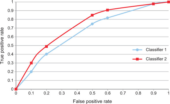
Figure 1.6 gives what is known as the receiver operating characteristic (ROC) curve of two imaginary classifiers. This curve traces the TPR and FPR as we twist our conceptual knob, thereby changing the parameters of the classifier. As mentioned previously, the ideal is a classifier with TPR=1 and TNR=1 (FPR=0); thus models that trace a line closer to the top-left corner of the graph are conceptually better, because they do a better job at separating negative and positive classes correctly. In this graph, classifier 2 clearly does a better job and should be chosen over classifier 1. Another way to encode this performance is by looking at the area under the ROC curve, sometimes known as the AUC (area under the curve). The larger the AUC, the better the performance of the model.
So far, so sensible! Be aware, however, that for predictive analytics solutions, things may not always be so easy. Take, for example, the issue of credit scoring. When you provide a score, you may not always be able to follow up on the behavior of that user in the future. Also, in these cases you’re usually not attempting to provide the answer but rather some indicator that’s correlated with a target variable (such as creditworthiness). Although the ROC curve can be used in these cases, there can be a few more hoops to jump through to get there.
1.7. Important notes about intelligent algorithms
Thus far we’ve covered a lot of introductory material. By now, you should have a fairly good, albeit high-level, understanding of intelligent algorithms and how you’re going to use them. You’re probably sufficiently motivated and anxious to dive into the details. We won’t disappoint you. Every following chapter is loaded with new and valuable code. But before we embark on our journey into the exciting and (for the more cynical among us) financially rewarding world of intelligent applications, we’ll present some useful things to know, many of which have been adapted from Pedro Domingos’s excellent and easy-to-read paper on the subject.[18] These should help guide you as you progress through this book and, later on, the field of intelligent algorithms.
Pedro Domingos, “A Few Useful Things to Know About Machine Learning,” Communications of the ACM 55, no. 10 (2012): 78–87.
1.7.1. Your data is not reliable
Your data may be unreliable for many reasons. That’s why you should always examine whether the data you’ll work with can be trusted before you start considering specific intelligent-algorithmic solutions to your problem. Even intelligent people who use very bad data will typically arrive at erroneous conclusions. The following is an indicative but incomplete list of the things that can go wrong with your data:
- The data that you have available during development may not be representative of the data that corresponds to a production environment. For example, you may want to categorize the users of a social network as “tall,” “average,” or “short” based on their height. If the shortest person in your development data is 6 feet tall (about 184 cm), you’re running the risk of calling someone short because they’re “just” 6 feet tall.
- Your data may contain missing values. In fact, unless your data is artificial, it’s almost certain to contain missing values. Handling missing values is a tricky business. Typically, you either leave the missing values or fill them in with some default or calculated values. Both conditions can lead to unstable implementations.
- Your data may change. The database schema may change, or the semantics of the data in the database may change.
- Your data may not be normalized. Let’s say that you’re looking at the weight of a set of individuals. In order to draw any meaningful conclusions based on the value of the weight, the unit of measurement should be the same for all individuals—pounds or kilograms for every person, not a mix of measurements in pounds and kilograms.
- Your data may be inappropriate for the algorithmic approach you have in mind. Data comes in various shapes and forms, known as data types. Some datasets are numeric, and some aren’t. Some datasets can be ordered, and some can’t. Some numeric datasets are discrete (such as the number of people in a room), and some are continuous (for example, the temperature or the atmospheric pressure).
1.7.2. Inference does not happen instantaneously
Computing a solution takes time, and the responsiveness of your application may be crucial for the financial success of your business. You shouldn’t assume that all algorithms on all datasets will run within the response-time limits of your application. You should test the performance of your algorithm within the range of your operating characteristics.
1.7.3. Size matters!
When we talk about intelligent applications, size does matter! The size of your data comes into the picture in two ways. The first is related to the responsiveness of the application, as mentioned earlier. The second is related to your ability to obtain meaningful results on a large dataset. You may be able to provide excellent movie or music recommendations for a set of users when the number of users is around 100, but the same algorithm may result in poor recommendations when the number of users involved is around 100,000.
Second, subject to the curse of dimensionality (covered in chapter 2), getting more data to throw at a simple algorithm often yields results that are far superior to making your classifier more and more complicated. If you look at large corporations such as Google, which use massive amounts of data, an equal measure of achievement should be attributed to how they deal with large volumes of training data as well as the complexity and sophistication of their classification solutions.
1.7.4. Different algorithms have different scaling characteristics
Don’t assume that an intelligent-application solution can scale just by adding more machines. Don’t assume that your solution is scalable. Some algorithms are scalable, and others aren’t. Let’s say that you’re trying to find groups of news stories with similar headlines among billions of titles. Not all clustering algorithms can run in parallel. You should consider scalability during the design phase of your application. In some cases, you may be able to split the data and apply your intelligent algorithm on smaller datasets in parallel. The algorithms you select in your design may have parallel (concurrent) versions, but you should investigate this from the outset, because typically you’ll build a lot of infrastructure and business logic around your algorithms.
1.7.5. Everything is not a nail!
You may have heard the phrase, “When all you have is a hammer, everything looks like a nail.” Well, we’re here to tell you that all of your intelligent-algorithm problems can’t be solved with the same algorithm!
Intelligent-application software is like every other piece of software—it has a certain area of applicability and certain limitations. Make sure you test your favorite solution thoroughly in new areas of application. In addition, it’s recommended that you examine every problem with a fresh perspective; a different algorithm may solve a different problem more efficiently or more expediently.
1.7.6. Data isn’t everything
Ultimately, ML algorithms aren’t magic, and they require an inductive step that allows you to reach outside the training data and into unseen data. For example, if you already know much regarding the dependencies of the data, a good representation may be graphical models—which can easily express this prior knowledge.[19] Careful consideration of what’s already known about the domain, along with the data, helps you build the most appropriate classifiers.
Judea Pearl, Probabilistic Reasoning in Intelligent Systems (Morgan Kaufmann Publishers, 1988).
1.7.7. Training time can be variable
In certain applications, it’s possible to have a large variance in solution times for a relatively small variation of the parameters involved. Typically, people expect that when they change the parameters of a problem, the problem can be solved consistently with respect to response time. If you have a method that returns the distance between any two geographic locations on Earth, you expect that the solution time will be independent of any two specific geographic locations. But this isn’t true for all problems. A seemingly innocuous change in the data can lead to significantly different solution times; sometimes the difference can be hours instead of seconds!
1.7.8. Generalization is the goal
One of the most common pitfalls with practitioners of ML is to get caught up in the process and to forget the final goal—to generalize the process or phenomenon under investigation. At the testing phase, it’s crucial to employ methods that allow you to investigate the generality of your solution (hold out test data, cross validate, and so on), but there’s no substitute for having an appropriate dataset to start with! If you’re trying to generalize a process with millions of attributes but only a few hundred test examples, chasing a percentage accuracy is tantamount to folly.
1.7.9. Human intuition is problematic
As the feature space grows, there’s a combinatorial explosion in the number of values the input may take. This makes it extremely unlikely that for any moderate-sized feature set you’ll see even a decent fraction of the total possible inputs. More worrisome, your intuition breaks down as the number of features increases. For example, in high dimensions, counter to intuition, most of the mass of a multivariate Gaussian distribution isn’t near the mean but in a “shell” around it.[20] Building simple classifiers in a low number of dimensions is easy, but increasing the number of dimensions makes it hard to understand what’s happening.
Domingos, “A Few Useful Things to Know About Machine Learning.”
1.7.10. Think about engineering new features
You’ve probably heard the phrase “garbage in, garbage out.” This is especially important when it comes to building solutions using ML approaches. Understanding the problem domain is key here, and deriving a set of features that exposes the underlying phenomena under investigation can mean all the difference to classification accuracy and generalization. It’s not good enough to throw all of your data at a classifier and hope for the best!
1.7.11. Learn many different models
Model ensembles are becoming increasingly common, due to their ability to reduce the variance of a classification with only a small cost to the bias. In the Netflix Prize, the overall winner and runner-up recommenders were both stacked (in which the output of each classifier is passed to a higher-level classifier) ensembles of more than 100 learners. Many believe that future classifiers will become more accurate through such techniques, but it does provide an additional layer of indirection for the non-expert to understand the mechanics of such a system.
1.7.12. Correlation is not the same as causation
This often-labored point is worth reiterating—and can be illustrated by a tongue-in-cheek thought experiment stating, ”Global warming, earthquakes, hurricanes, and other natural disasters are a direct effect of the shrinking numbers of pirates since the 1800s.”[21] Just because two variables are correlated, this doesn’t imply causation between the two. Often there is a third (or fourth or fifth!) variable that isn’t observable and is at play. Correlation should be taken as a sign of potential causation, warranting further investigation.
Bobby Henderson, “An Open Letter to Kansas School Board,” Verganza (July 1, 2005), www.venganza.org/about/open-letter.
1.8. Summary
- We provided the 50,000–foot view of intelligent algorithms, providing many specific examples based on real-world problems.
- An intelligent algorithm is any that can modify its behavior based on incoming data.
- We provided some intelligent-algorithm design anti-patterns that will hopefully serve as a warning flag for practitioners in the space.
- You’ve seen that intelligent algorithms can be broadly divided into three categories: artificial intelligence, machine learning, and predictive analytics. We’ll spend the most time on the latter two in this book, so if you glanced over these sections, it would be worth rereading them to ensure good foundational knowledge.
- We introduced some key metrics such as the receiver operating characteristic. The area under the ROC curve is often used to assess the relative performance of models. Be warned that there are many ways to evaluate performance, and here we only introduced the basics.
- We provided you with some useful facts that have been learned collectively by the intelligent-algorithm community. These can provide an invaluable compass by which to navigate the field.