The amount of data that’s generated increases every day. Technology advances have facilitated the storage of huge amounts of data. This data deluge has forced users to adopt distributed systems. Distributed systems look for distributed programming, which requires extra care for fault tolerance and efficient algorithms. Distributed systems always look for two things—reliability of the system and availability of all the components.
Apache Hadoop ensures efficient computation and fault tolerance for distributed systems. Mainly it concentrates on reliability and availability. Apache Hadoop is easy to program, therefore many became interested in Big Data. E-commerce companies wanted to know more about their customers; the healthcare industry wanted to know insights from their data; and other industries were interested in knowing more about the data they were capturing. More data metrics were defined and more data points were collected.
Many open source Big Data tools emerged, including Apache Tez and Apache Storm . Many NoSQL databases also emerged to deal with huge data inflow. Apache Spark also evolved as a distributed system and became very popular over time.
This chapter discusses Big Data and Hadoop as a distributed system to process Big Data. We will also cover the Hadoop ecosystem frameworks, like Apache Hive and Apache Pig. We also throw light on the shortcomings of Hadoop and will discuss the development of Apache Spark. Then we will cover Apache Spark. We also discuss the different cluster managers that work with Apache Spark. We discuss PySpark SQL, which is the core of this book and its usefulness. Without discussing NoSQL, this chapter is not justified. So a discussion of the NoSQL databases, MongoDB and Cassandra, is included in this chapter. Sometimes we read data from Relational Database Management Systems (RDBMSs) as well, so this chapter discusses PostgreSQL.
Introduction to Big Data
Big Data is one of the hottest topics of this era. But what is this Big Data? It describes a dataset that’s huge and is increasing with amazing speed. Apart from its volume and the velocity, Big Data is also characterized by the variety of data and its veracity. Let’s discuss volume, velocity, variety, and veracity in detail. These are also known as the 4V characteristics of Big Data.
Volume
Data volume specifies the amount of data to be processed. For large amounts of data, we need large machines or distributed systems. The time of computation increases with the volume of data. So it’s better to use a distributed system if we can parallelize our computation. The volume might be of structured data, unstructured data, or something in between. If we have unstructured data, then the situation becomes more complex and computatively intensive. You might wonder, how big is Big Data? This is a debatable question. But in a general way, we can say that the amount of data that we can’t handle using a conventional system is defined as Big Data. Now let’s discuss the velocity of data.
Velocity
Organizations are becoming more and more data conscious. A large amount of data is collected every moment. This means that the velocity of the data is increasing. How can a single system handle this velocity? The problem becomes complex when you have to analyze large inflows of data in real time. Many systems are being developed to deal with this huge inflow of data. Another component that differentiates conventional data from Big Data is the variety of data, discussed next.
Variety
The variety of data can make it so complex that conventional data analysis systems cannot analyze it properly. What kind of variety are we talking about? Isn’t data just data? Image data is different than tabular data, because of the way it is organized and saved. Infinite numbers of filesystems are available. Every filesystem requires a different way of dealing with it. Reading and writing a JSON file is different than the way we deal with a CSV file. Nowadays, a data scientist has to deal with combinations of datatypes. The data you are going to deal with might be a combination of pictures, videos, text, etc. The variety of Big Data makes it more complex to analyze.
Veracity

Big Data
Introduction to Hadoop
“MapReduce: Simplified Data Processing on Large Clusters,” by Jeffrey Dean and Sanjay Ghemawat
“The Google File System,” by Sanjay Ghemawat, Howard Gobioff, and Shun-Tak Leung
Working on commodity hardware makes it very cost effective. If we are working on commodity hardware, faults are an inevitable issue. But Hadoop provides a fault-tolerant system for data storage and computation. This fault-tolerant capability made Hadoop very popular.

Hadoop components
Introduction to HDFS
HDFS is used to store large amounts of data in a distributed and fault-tolerant fashion. HDFS is written in Java and runs on commodity hardware. It was inspired by the Google research paper of the Google File System (GFS). It is a write once and read many times system, and it’s effective for large amounts of data.
HDFS has two components—NameNode and DataNode. These two components are Java daemon processes. A NameNode, which maintains meta data of files distributed on a cluster, work as masters for many DataNodes. HDFS divides a large file into small blocks and saves the blocks on different DataNodes. Actual file data blocks reside on DataNodes.
HDFS provides a set of UNIX-shell like commands. But we can use the Java filesystem API provided by HDFS to work at a finer level on large files. Fault tolerance is implemented using replication of data blocks.

Components of HDFS
Introduction to MapReduce
The MapReduce model of computation first appeared in a research paper by Google. This research paper was implemented in Hadoop as Hadoop’s MapReduce. Hadoop’s MapReduce is a computation engine of the Hadoop Framework, which does computations on distributed data in HDFS. MapReduce has been found horizontally scalable on distributed systems of commodity hardware. It also scales up for large problems. In MapReduce, the problem solution is broken into two phases—the Map phase and the Reduce phase. In the Map phase, chunks of data are processed and in the Reduce phase, aggregation or reduction operations run on the results from the Map phase. Hadoop’s MapReduce framework was written in Java.
MapReduce is a master-slave model. In Hadoop 1, this MapReduce computation was managed by two daemon processes—Jobtracker and Tasktracker. Jobtracker is master process that deals with many Tasktrackers. Tasktracker is a slave to Jobtracker. But in Hadoop 2, Jobtracker and Tasktracker were replaced by YARN.
Hadoop’s MapReduce framework was written in Java. We can write our MapReduce code using the API provided by the framework and in Java. The Hadoop streaming module enables programmers with Python and Ruby knowledge to program MapReduce.
MapReduce algorithms have many uses. Many machine learning algorithms were implemented as Apache Mahout, which runs on Hadoop as Pig and Hive.
But MapReduce is not very good for iterative algorithms. At the end of every Hadoop job, MapReduce saves the data to HDFS and reads it back again for the next job. We know that reading and writing data to files are costly activities. Apache Spark mitigated the shortcomings of MapReduce by providing in-memory data persistence and computation.
Note
You can read more about MapReduce and Mahout on the following web pages
Introduction to Apache Hive
Computer science is a world of abstraction. Everyone knows that data is information in the form of bits. Programming languages like C provide abstraction over the machine and assembly language. More abstraction is provided by other high-level languages. Structured Query Language (SQL) is one of those abstractions. SQL is used all over the world by many data modeling experts. Hadoop is good for Big Data analysis. So how can a large population, knowing SQL, utilize the power of Hadoop computational power on Big Data? In order to write Hadoop's MapReduce program, users must know a programming language that can be used to program Hadoop’s MapReduce.
Real world day-to-day problems follow certain patterns. Some problems are common in day-to-day life, such as manipulation of data, handling missing values, data transformation, and data summarization. Writing MapReduce code for these day-to-day problems is great head-spinning work for non-programmers. Writing code to solve a problem is not a very intelligent thing. But writing efficient code that has performance scalability and can be extended is valuable. With this problem in mind, Apache Hive was developed at Facebook, so that day-to-day problems could be solved without having to write MapReduce code for general problems.
According to the language of the Hive wiki, “Hive is a data warehousing infrastructure based on Apache Hadoop”. Hive has its own SQL dialect, known as the Hive Query Language. It is known as HiveQL or sometimes HQL. Using HiveQL, Hive queries data in HDFS. Hive not only runs on HDFS but it runs on Spark too and other Big Data frameworks like Apache Tez.
Hive provides a Relational Database Management System-like abstraction to users for structured data in HDFS. You can create tables and run SQL-like queries on them. Hive saves the table schema in some RDBMS. Apache Derby is the default RDBMS that ships with the Apache Hive distribution. Apache Derby has been fully written in Java and is an open source RDBMS that comes with Apache License Version 2.0.
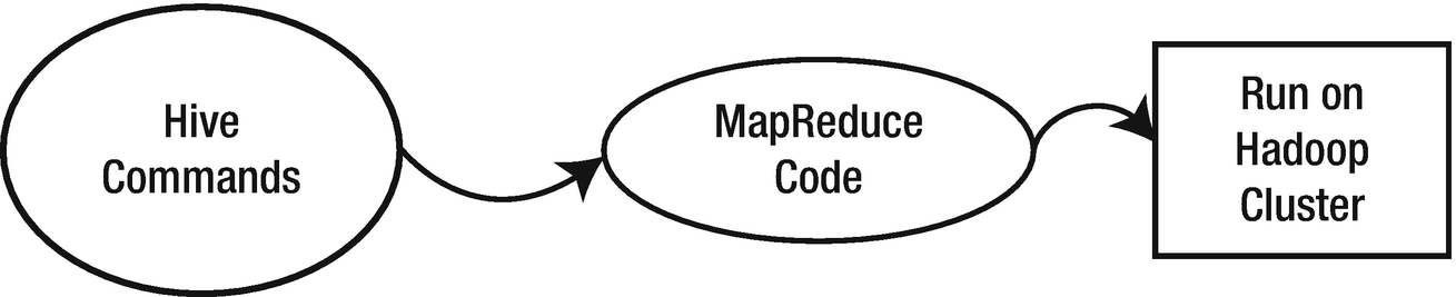
Code execution flow in Apache Hive
A person knowing SQL can easily learn Apache Hive and HiveQL and can use the storage and computation power of Hadoop in their day-to-day data analysis jobs on Big Data. HiveQL is also supported by PySpark SQL. You can run HiveQL commands in PySpark SQL. Apart from executing HiveQL queries, you can also read data from Hive directly to PySpark SQL and write results to Hive. See Figure 1-4.
Note
You can read more about Hive and Apache Derby RDBMS from the following web pages
Introduction to Apache Pig
Apache Pig is data flow framework for performing data analysis on a huge amount of data. It was developed by Yahoo!, and it was open sourced to Apache Software Foundation. It’s now available under Apache License Version 2.0. The Pig programming language is a Pig Latin scripting language. Pig is loosely connected to Hadoop, which means that we can connect it to Hadoop and perform many analysis. But Pig can be used with other tools like Apache Tez and Apache Spark.
Apache Hive is used as a reporting tool where Apache Pig is used to extract, transform, and load (ETL). We can extend the functionality of Pig using user-defined functions (UDF). User-defined functions can be written in many languages, including Java, Python, Ruby, JavaScript, Groovy, and Jython.

Code execution flow in Apache Pig
The best part of Pig is that the code is optimized and tested to work with day-to-day problems. So users can directly install Pig and start using it. Pig provides the Grunt shell to run interactive Pig commands. So anyone who knows Pig Latin can enjoy the benefits of HDFS and MapReduce, without knowing advanced programming languages like Java or Python.
Introduction to Apache Kafka
Apache Kafka is a publish-subscribe, distributed messaging platform. It was developed at LinkedIn and further open sourced to the Apache foundation. It is fault tolerant, scalable, and fast. Messages in Kafka terms, which is the smallest unit of data, flow from producer to consumer through the Kafka Server, and can be persisted and used at a later time. You might be confused about the terms producer and consumer. We are going to discuss these terms very soon. Another key term we are going to use in the context of Kafka is topic. A topic is a stream of messages of a similar category. Kafka comes with a built-in API that developers can use to build their applications. We are the ones who define the topic. Next we discuss the three main components of Apache Kafka.
Producer
The Kafka producer produces the message to a Kafka topic. It can publish data to more than one topic.
Broker
This is the main Kafka server that runs on a dedicated machine. Messages are pushed to the broker by the producer. The broker persists topics in different partitions and these partitions are replicated to different brokers to deal with faults. It is stateless in nature, therefore the consumer has to track the message it consumes.
Consumer
The consumer fetches the message from the Kafka Broker. Remember, it fetches the messages. The Kafka Broker is not pushing messages to the consumer; rather, the consumer is pulling data from the Kafka Broker. Consumers are subscribed to one or more topics on the Kafka Broker and they read the messages. The broker also keeps tracks of all the messages it has consumed. Data is persisted in the broker for a specified time. If the consumer fails, it can fetch the data after it restarts.

Apache Kafka message flow
We will integrate Apache Kafka with PySpark in Chapter 7 and discuss Kafka in more detail.
Introduction to Apache Spark
Apache Spark is a general purpose, distributed programming framework. It is considered very good for iterative as well as batch processing data. It was developed at the AMP lab. It provides an in-memory computation framework. It is open source software. On the one hand, it is best with batch processing, and on the other hand, it works very well with real-time or near real-time data. Machine learning and graph algorithms are iterative in nature and this is where Spark does its magic. According to its research paper, it is much faster than its peer, Hadoop. Data can be cached in memory. Caching intermediate data in iterative algorithms provides amazingly fast processing. Spark can be programmed using Java, Scala, Python, and R.
“Resilient Distributed Datasets: A Fault-Tolerant Abstraction for In-Memory Cluster Computing,” by Matei Zaharia, Mosharaf Chowdhury, Tathagata Das, Ankur Dave, Justin Ma, Murphy McCauley, Michael J. Franklin, Scott Shenker, and Ion Stoica.
“Spark: Cluster Computing with Working Sets,” by Matei Zaharia, Mosharaf Chowdhury, Michael J. Franklin, Scott Shenker, and Ion Stoica.
“MLlib: Machine Learning in Apache Spark,” by Xiangrui Meng, Joseph Bradley, Burak Yavuz, Evan Sparks, Shivaram Venkataraman, Davies Liu, Jeremy Freeman, DB Tsai, Manish Amde, Sean Owen, Doris Xin, Reynold Xin, Michael J. Franklin, Reza Zadeh, Matei Zaharia, and Ameet Talwalkar.
If you consider Spark as improved Hadoop, up to some extent, this is fine in my view. Because we can implement the MapReduce algorithm in Spark, Spark uses the benefit of HDFS. That means it can read data from HDFS and store data to HDFS, and it handles iterative computation efficiently because data can be persisted in memory. Apart from in-memory computation, it is good for interactive data analysis.
MLlib: MLlib is a wrapper over the PySpark core, and it deals with machine learning algorithms. The machine learning APIs provided by the MLlib library are very easy to use. MLlib supports many machine learning algorithms of classification, clustering, text analysis, and many more.
ML: ML is also a machine learning library that sits on the PySpark core. Machine learning APIs of ML can work on DataFrames.
GraphFrames : The GraphFrames library provides a set of APIs to do graph analysis efficiently using PySpark core and PySpark SQL. At the time of writing this book, DataFrames is an external library. You have to download and install it separately.
PySpark SQL: An Introduction
Most data that data scientists deal with is either structured or semi-structured in nature. The PySpark SQL module is a higher level abstraction over that PySpark core in order to process structured and semi-structured datasets. We are going to study PySpark SQL throughout the book. It comes built into PySpark, which means that it does not require any extra installation.
PySpark SQL can be programmed using a domain-specific language. As in our case, we are going to use Python to program PySpark SQL. Apart from a domain-specific language, we can run Structured Query Language (SQL) and HiveQL queries. Using SQL and HiveQL makes PySpark SQL popular among database programmers and Apache Hive users.
Using PySpark SQL, you can read data from many sources. PySpark SQL supports reading from many file format systems, including text files, CSV, ORC, Parquet, JSON, etc. You can read data from Relational Database Management System (RDBMS), such as MySQL and PostgreSQL. You can save the analysis report to many systems and file formats too.
PySpark SQL introduced DataFrames, which create tabular representations of structured data and provide tables in RDBMS. Another data abstraction dataset was introduced in Spark 1.6, but it does not work with PySpark SQL.
Introduction to DataFrames
DataFrames are an abstraction similar to tables in Relational Database Systems. They consist of named columns. DataFrames are collections of row objects, which are defined in PySpark SQL. DataFrames consist of named column objects as well. Users know the schema of the tabular form, so it becomes easy to operate on DataFrames.
DataFrames
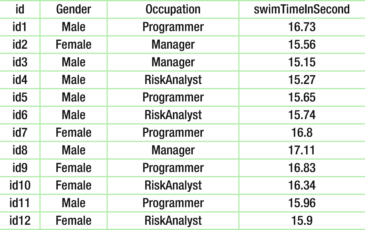
Figure 1-7 depicts a DataFrame with four columns. The name of the columns are id, Gender, Occupation, and swimTimeInSecond. The datatype of the first three columns is String, whereas the last column contains floating-point data. The DataFrame has two components—the data and its schema. It should be clear that this is similar to RDBMS tables or R programming DataFrames .
Note
Datasets are not used in PySpark. The interested reader can read about datasets and their APIs at the following link
https://spark.apache.org/docs/latest/sql-programming-guide.html
SparkSession
A SparkSession object is the entry point that replaced SQLContext and HiveContext. To make PySpark SQL code compatible with previous versions, SQLContext and HiveContext continue in PySpark. In the PySpark console, we get the SparkSession object. We can create a SparkSession object using the following code.
The appName function will set the name of the application. The getOrCreate() function will return an existing SparkSession object. If no SparkSession object exists, the getOrCreate() function will create a new object and return it.
Structured Streaming
We can stream data analysis using the Structured Streaming framework, which is a wrapper over PySpark SQL. We can perform analysis on streaming data in a similar fashion using Structured Streaming as we perform batch analysis on static data using PySpark SQL.
Just as the Spark streaming module performs streaming operations on mini-batches, the Structured Streaming engine performs streaming operations on mini-batches.
The best part of structured streaming is that it uses a similar API as for PySpark SQL. Therefore, the learning curve is high. Operations on DataFrames are optimized and, in a similar fashion, the Structured Streaming API is optimized in the context of performance.
Catalyst Optimizer
SQL is a declarative language. Using SQL, we tell the SQL engine what to do. We do not tell it how to perform the task. Similarly, PySpark SQL commands do not tell it how to perform a task. These commands only tell it what to perform. So, the PySpark SQL queries require optimization while performing tasks. The catalyst optimizer performs query optimization in PySpark SQL. The PySpark SQL query is transformed into low-level Resilient Distributed Dataset (RDD) operations. The catalyst optimizer first transforms the PySpark SQL query to a logical plan and then transforms this logical plan to an optimized logical plan. From this optimized logical plan, a physical plan is created. More than one physical plan is created. Using a cost analyzer, the most optimized physical plan is selected. And finally, low-level RDD operation code is created.
Introduction to Cluster Managers
In a distributed system, a job or application is broken into different tasks, which can run in parallel on different machines in the cluster. If the machines fail, you have to reschedule the task on another machine.
The distributed system generally faces scalability problems due to mismanagement of resources. Consider a job that’s already running on a cluster. Another person wants to run another job. That second job has to wait until the first is finished. But in this way we are not utilizing the resources optimally. Resource management is easy to explain but difficult to implement on a distributed system. Cluster managers were developed to manage cluster resources optimally. There are three cluster managers available for Spark—standalone, Apache Mesos, and YARN. The best part of these cluster managers is that they provide an abstraction layer between users and clusters. The user experience is like working on a single machine, although they are working on a cluster, due to the abstraction provided by the cluster managers. Cluster managers schedule cluster resources to running applications.
Standalone Cluster Manager
Apache Spark ships with a standalone cluster manager. It provides a master-slave architecture to Spark clusters. It is a Spark-only cluster manager. You can run only Spark applications using this standalone cluster manager. Its components are the master and the workers. Workers are slaves to the master process. It is the simplest cluster manager. The Spark standalone cluster manager can be configured using scripts in the sbin directory of Spark. We will configure the Spark standalone cluster manager in coming chapters and will deploy PySpark applications using the standalone cluster manager.
Apache Mesos Cluster Manager
Apache Mesos is a general purpose cluster manager. It was developed at the University of California, Berkeley AMP lab. Apache Mesos helps distributed solutions to scale efficiently. You can run different applications using different frameworks on the same cluster using Mesos. What is the meaning of different applications from different frameworks? This means that you can run a Hadoop application and a Spark application simultaneously on Mesos. While multiple applications are running on Mesos, they share the resources of the cluster. Apache Mesos has two important components—the master and slaves. This master-slaves architecture is similar to the Spark Standalone cluster manager. The applications running on Mesos are known as frameworks. Slaves tell the master about the resources available to it as a resource offer. The slave machine provides resource offers periodically. The allocation module of the master server decides which framework gets the resources.
YARN Cluster Manager
YARN stands for “Yet Another Resource Negotiator”. YARN was introduced in Hadoop 2 to scale Hadoop. Resource management and job management were separated. Separating these two components made Hadoop scale better. YARN’s main components are the ResourceManager, ApplicationMaster, and NodeManager. There is one global ResourceManager and many NodeManagers will be running per cluster. NodeManagers are slaves to the ResourceManager. The Scheduler, which is a component of the ResourceManager, allocates resources for different applications working on clusters. The best part is that you can run a Spark application and any other applications like Hadoop or MPI simultaneously on clusters managed by YARN . There is one ApplicationMaster per application, and it deals with the task running in parallel on the distributed system. Remember, Hadoop and Spark have their own ApplicationMaster.
Note
You can read more about standalone, Apache Mesos, and YARN cluster managers on the following web pages.
https://spark.apache.org/docs/2.0.0/spark-standalone.html
Introduction to PostgreSQL
Relational Database Management Systems are still very common in many organizations. What is the meaning of relation here? Relation means tables. PostgreSQL is a Relational Database Management System. It runs on all major operating systems like Microsoft Windows, UNIX-based operating systems, MacOS X, and many more. It is an open source program and the code is available under the PostgreSQL license. Therefore, you can use it freely and modify it according to your requirements.
PostgreSQL databases can be connected through other programming languages like Java, Perl, Python, C, and C++, and many other languages through different programming interfaces. It can be also be programmed using a procedural programming language called PL/pgSQL (Procedural Language/PostgreSQL) , which is similar to PL/SQL. You can add custom functions to this database. You can write custom functions in C/C++ and other programming languages. You can also read data from PostgreSQL from PySpark SQL using JDBC connectors. In the coming chapters, we are going to read data tables from PostgreSQL using PySpark SQL. We are also going to explore some more facets of PostgreSQL in coming chapters.
PostgreSQL follows the ACID (Atomicity, Consistency, Isolation and Durability) principles. It comes with many features, some of which are unique to PostgreSQL. It supports updatable views, transactional integrity, complex queries, triggers, and others. PostgreSQL does its concurrency management using the multi-version concurrency control model.
There is wide community support for PostgreSQL. PostgreSQL has been designed and developed to be extensible.
Note
If you want to learn about PostgreSQL in depth, the following links will be very helpful.
https://wiki.postgresql.org/wiki/Main_Page
https://en.wikipedia.org/wiki/PostgreSQL
https://en.wikipedia.org/wiki/Multiversion_concurrency_control
Introduction to MongoDB
MongoDB is a document-based NoSQL database. It is an open source, distributed database, which was developed by MongoDB Inc. MongoDB is written in C++ and it scales horizontally. It is being used by many organizations for backend databases and for many other purposes.
MongoDB comes with a mongo shell, which is a JavaScript interface to the MongoDB server. The mongo shell can be used to run queries as well as perform administrative tasks. On the mongo shell, we can run JavaScript code too.
Using PySpark SQL, we can read data from MongoDB and perform analyses. We can also write the results.
Introduction to Cassandra
Cassandra is open source, distributed database that comes with the Apache License. It is a NoSQL database developed at Facebook. It is horizontally scalable and works best with structured data. It provides a high level of consistency and has tunable consistency. It does not have a single point of failure. It replicates data on different nodes with a peer-to-peer distributed architecture. Nodes exchange their information using the gossip protocol.
Note
You can read more about Apache Cassandra from the following links