Chapter 3. Draw
At first, drawing on a computer screen is like working on graph paper. It starts as a careful technical procedure, but as new concepts are introduced, drawing simple shapes with software expands into animation and interaction. Before we make this jump, we need to start at the beginning.
A computer screen is a grid of light elements called pixels. Each pixel has a position within the grid defined by coordinates. In Processing, the x coordinate is the distance from the left edge of the Display Window and the y coordinate is the distance from the top edge. We write coordinates of a pixel like this: (x, y). So, if the screen is 200×200 pixels, the upper-left is (0, 0), the center is at (100, 100), and the lower-right is (199, 199). These numbers may seem confusing; why do we go from 0 to 199 instead of 1 to 200? The answer is that in code, we usually count from 0 because it’s easier for calculations that we’ll get into later.
The Display Window
The Display Window is created and images are drawn inside through code elements called functions. Functions are the basic building blocks of a Processing program. The behavior of a function is defined by its parameters. For example, almost every Processing program has a size() function to set the width and height of the Display Window. (If your program doesn’t have a size() function, the dimension is set to 100×100 pixels.)
Example 3-1: Draw a Window
The size() function has two parameters: the first sets the width of the window and the second sets the height. To draw a window that is 800 pixels wide and 600 high, type:
size(800,600);
Run this line of code to see the result. Put in different values to see what’s possible. Try very small numbers and numbers larger than your screen.
Example 3-2: Draw a Point
To set the color of a single pixel within the Display Window, we use the point() function. It has two parameters that define a position: the x coordinate followed by the y coordinate. To draw a little window and a point at the center of the screen, coordinate (240, 60), type:

size(480,120);point(240,60);
Try to write a program that puts a point at each corner of the Display Window and one in the center. Try placing points side by side to make horizontal, vertical, and diagonal lines.
Basic Shapes
Processing includes a group of functions to draw basic shapes (see Figure 3-1). Simple shapes like lines can be combined to create more complex forms like a leaf or a face.
To draw a single line, we need four parameters: two for the starting location and two for the end.
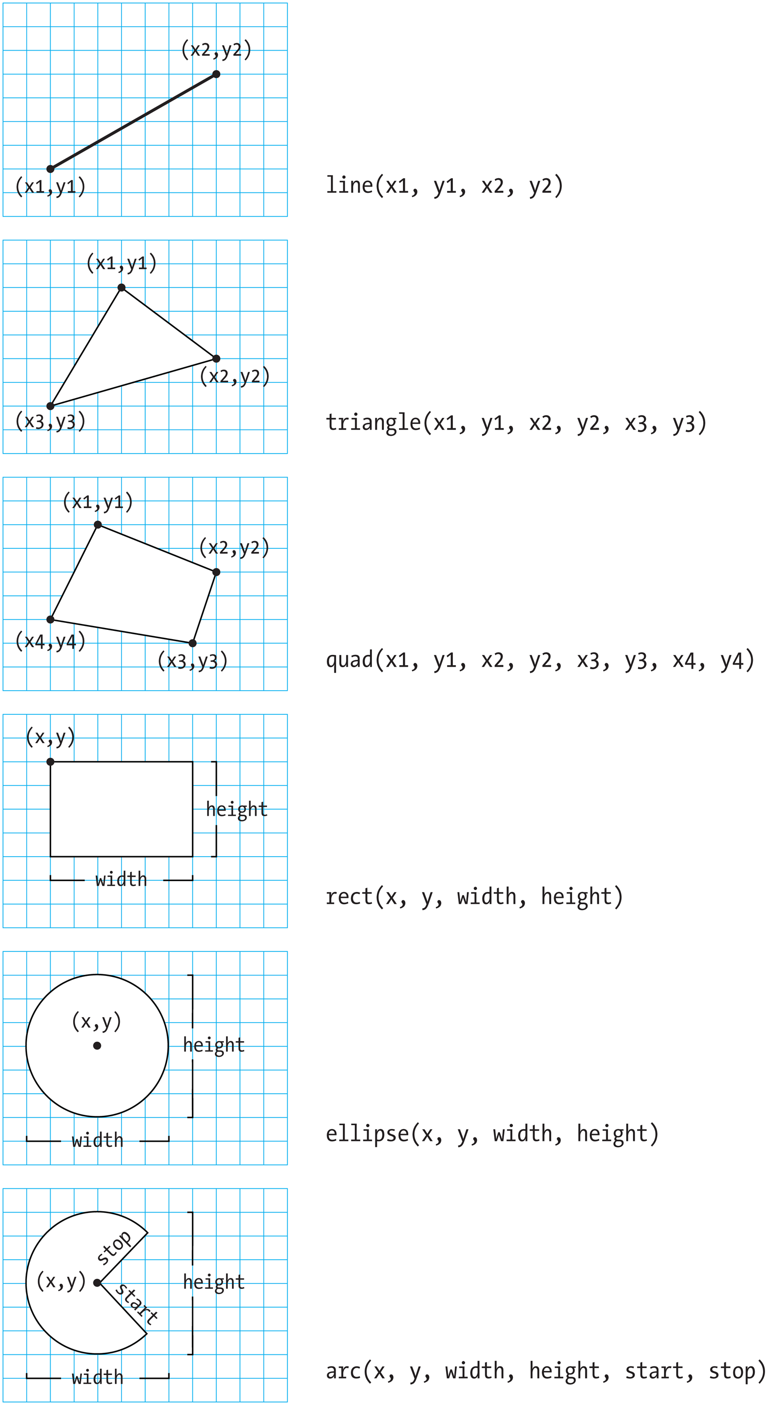
Figure 3-1. Shapes and their coordinates
Example 3-3: Draw a Line
To draw a line between coordinate (20, 50) and (420, 110), try:

size(480,120);line(20,50,420,110);

Example 3-5: Draw a Rectangle
Rectangles and ellipses are both defined with four parameters: the first and second are for the x and y coordinates of the anchor point, the third for the width, and the fourth for the height. To make a rectangle at coordinate (180, 60) with a width of 220 pixels and height of 40, use the rect() function like this:

size(480,120);rect(180,60,220,40);
Example 3-6: Draw an Ellipse
The x and y coordinates for a rectangle are the upper-left corner, but for an ellipse they are the center of the shape. In this example, notice that the y coordinate for the first ellipse is outside the window. Objects can be drawn partially (or entirely) out of the window without an error:

size(480,120);ellipse(278,-100,400,400);ellipse(120,100,110,110);ellipse(412,60,18,18);
Processing doesn’t have separate functions to make squares and circles. To make these shapes, use the same value for the width and the height parameters to ellipse() and rect().
Example 3-7: Draw Part of an Ellipse
The arc() function draws a piece of an ellipse:

size(480,120);arc(90,60,80,80,0,HALF_PI);arc(190,60,80,80,0,PI+HALF_PI);arc(290,60,80,80,PI,TWO_PI+HALF_PI);arc(390,60,80,80,QUARTER_PI,PI+QUARTER_PI);
The first and second parameters set the location, the third and fourth set the width and height. The fifth parameter sets the angle to start the arc, and the sixth sets the angle to stop. The angles are set in radians, rather than degrees. Radians are angle measurements based on the value of pi (3.14159). Figure 3-2 shows how the two relate. As featured in this example, four radian values are used so frequently that special names for them were added as a part of Processing. The values PI, QUARTER_PI, HALF_PI, and TWO_PI can be used to replace the radian values for 180°, 45°, 90°, and 360°.

Figure 3-2. Radians and degrees are two ways to measure an angle. Degrees move around the circle from 0 to 360, while radians measure the angles in relation to pi, from 0 to approximately 6.28.
Example 3-8: Draw with Degrees
If you prefer to use degree measurements, you can convert to radians with the radians() function. This function takes an angle in degrees and changes it to the corresponding radian value. The following example is the same as Example 3-7, but it uses the radians() function to define the start and stop values in degrees:
size(480,120);arc(90,60,80,80,0,radians(90));arc(190,60,80,80,0,radians(270));arc(290,60,80,80,radians(180),radians(450));arc(390,60,80,80,radians(45),radians(225));
Drawing Order
When a program runs, the computer starts at the top and reads each line of code until it reaches the last line and then stops. If you want a shape to be drawn on top of all other shapes, it needs to follow the others in the code.
Example 3-9: Control Your Drawing Order
size(480,120);ellipse(140,0,190,190);// The rectangle draws on top of the ellipse// because it comes after in the coderect(160,30,260,20);
Example 3-10: Put It in Reverse
Modify by reversing the order of rect() and ellipse() to see the circle on top of the rectangle:

size(480,120);rect(160,30,260,20);// The ellipse draws on top of the rectangle// because it comes after in the codeellipse(140,0,190,190);
You can think of it like painting with a brush or making a collage. The last element that you add is what’s visible on top.
Shape Properties
The most basic and useful shape properties are stroke weight, the way the ends (caps) of lines are drawn, and how the corners of shapes are displayed.
Example 3-11: Set Stroke Weight
The default stroke weight is a single pixel, but this can be changed with the strokeWeight() function. The single parameter to strokeWeight() sets the width of drawn lines:

size(480,120);ellipse(75,60,90,90);strokeWeight(8);// Stroke weight to 8 pixelsellipse(175,60,90,90);ellipse(279,60,90,90);strokeWeight(20);// Stroke weight to 20 pixelsellipse(389,60,90,90);
Example 3-12: Set Stroke Caps
The strokeCap() function changes how lines are drawn at their endpoints. By default, they have rounded ends:

size(480,120);strokeWeight(24);line(60,25,130,95);strokeCap(SQUARE);// Square the line endingsline(160,25,230,95);strokeCap(PROJECT);// Project the line endingsline(260,25,330,95);strokeCap(ROUND);// Round the line endingsline(360,25,430,95);
Example 3-13: Set Stroke Joins
The strokeJoin() function changes the way lines are joined (how the corners look). By default, they have pointed (mitered) corners:

size(480,120);strokeWeight(12);rect(60,25,70,70);strokeJoin(ROUND);// Round the stroke cornersrect(160,25,70,70);strokeJoin(BEVEL);// Bevel the stroke cornersrect(260,25,70,70);strokeJoin(MITER);// Miter the stroke cornersrect(360,25,70,70);
When any of these attributes are set, all shapes drawn afterward are affected. For instance, in Example 3-11, notice how the second and third circles both have the same stroke weight, even though the weight is set only once before both are drawn.
Drawing Modes
A group of functions with “mode” in their name change how Processing draws geometry to the screen. In this chapter, we’ll look at ellipseMode() and rectMode(), which help us to draw ellipses and rectangles, respectively; later in the book, we’ll cover imageMode() and shapeMode().
Example 3-14: On the Corner
By default, the ellipse() function uses its first two parameters as the x and y coordinate of the center and the third and fourth parameters as the width and height. After ellipseMode(CORNER) is run in a sketch, the first two parameters to ellipse() then define the position of the upper-left corner of the rectangle the ellipse is inscribed within. This makes the ellipse() function behave more like rect() as seen in this example:

size(480,120);rect(120,60,80,80);ellipse(120,60,80,80);ellipseMode(CORNER);rect(280,20,80,80);ellipse(280,20,80,80);
You’ll find these “mode” functions in examples throughout the book. There are more options for how to use them in the Processing Reference.
Color
All the shapes so far have been filled white with black outlines, and the background of the Display Window has been light gray. To change them, use the background(), fill(), and stroke() functions. The values of the parameters are in the range of 0 to 255, where 255 is white, 128 is medium gray, and 0 is black. Figure 3-3 shows how the values from 0 to 255 map to different gray levels.

Figure 3-3. Colors are created by defining RGB (red, green, blue) values
Example 3-15: Paint with Grays
This example shows three different gray values on a black background:

size(480,120);background(0);// Blackfill(204);// Light grayellipse(132,82,200,200);// Light gray circlefill(153);// Medium grayellipse(228,-16,200,200);// Medium gray circlefill(102);// Dark grayellipse(268,118,200,200);// Dark gray circle
Example 3-16: Control Fill and Stroke
You can disable the stroke so that there’s no outline by using noStroke(), and you can disable the fill of a shape with noFill():

size(480,120);fill(153);// Medium grayellipse(132,82,200,200);// Gray circlenoFill();// Turn off fillellipse(228,-16,200,200);// Outline circlenoStroke();// Turn off strokeellipse(268,118,200,200);// Doesn't draw!
Be careful not to disable the fill and stroke at the same time, as we’ve done in the previous example, because nothing will draw to the screen.
Example 3-17: Draw with Color
To move beyond grayscale values, you use three parameters to specify the red, green, and blue components of a color.
Run the code in Processing to reveal the colors:

size(480,120);noStroke();background(0,26,51);// Dark blue colorfill(255,0,0);// Red colorellipse(132,82,200,200);// Red circlefill(0,255,0);// Green colorellipse(228,-16,200,200);// Green circlefill(0,0,255);// Blue colorellipse(268,118,200,200);// Blue circle
This is referred to as RGB color, which comes from how computers define colors on the screen. The three numbers stand for the values of red, green, and blue, and they range from 0 to 255 the way that the gray values do. Using RGB color isn’t very intuitive, so to choose colors, use Tools→Color Selector, which shows a color palette similar to those found in other software (see Figure 3-4). Select a color, and then use the R, G, and B values as the parameters for your background(), fill(), or stroke() function.

Figure 3-4. Processing Color Selector
Example 3-18: Set Transparency
By adding an optional fourth parameter to fill() or stroke(), you can control the transparency. This fourth parameter is known as the alpha value, and also uses the range 0 to 255 to set the amount of transparency. The value 0 defines the color as entirely transparent (it won’t display), the value 255 is entirely opaque, and the values between these extremes cause the colors to mix on screen:

size(480,120);noStroke();background(204,226,225);// Light blue colorfill(255,0,0,160);// Red colorellipse(132,82,200,200);// Red circlefill(0,255,0,160);// Green colorellipse(228,-16,200,200);// Green circlefill(0,0,255,160);// Blue colorellipse(268,118,200,200);// Blue circle
Custom Shapes
You’re not limited to using these basic geometric shapes—you can also define new shapes by connecting a series of points.
Example 3-19: Draw an Arrow
The beginShape() function signals the start of a new shape. The vertex() function is used to define each pair of x and y coordinates for the shape. Finally, endShape() is called to signal that the shape is finished:

size(480,120);beginShape();fill(153,176,180);vertex(180,82);vertex(207,36);vertex(214,63);vertex(407,11);vertex(412,30);vertex(219,82);vertex(226,109);endShape();
Example 3-20: Close the Gap
When you run Example 3-19, you’ll see the first and last point are not connected. To do this, add the word CLOSE as a parameter to endShape(), like this:

size(480,120);beginShape();fill(153,176,180);vertex(180,82);vertex(207,36);vertex(214,63);vertex(407,11);vertex(412,30);vertex(219,82);vertex(226,109);endShape(CLOSE);
Example 3-21: Create Some Creatures
The power of defining shapes with vertex() is the ability to make shapes with complex outlines. Processing can draw thousands and thousands of lines at a time to fill the screen with fantastic shapes that spring from your imagination. A modest but more complex example follows:

size(480,120);// Left creaturefill(153,176,180);beginShape();vertex(50,120);vertex(100,90);vertex(110,60);vertex(80,20);vertex(210,60);vertex(160,80);vertex(200,90);vertex(140,100);vertex(130,120);endShape();fill(0);ellipse(155,60,8,8);// Right creaturefill(176,186,163);beginShape();vertex(370,120);vertex(360,90);vertex(290,80);vertex(340,70);vertex(280,50);vertex(420,10);vertex(390,50);vertex(410,90);vertex(460,120);endShape();fill(0);ellipse(345,50,10,10);
Comments
The examples in this chapter use double slashes (//) at the end of a line to add comments to the code. Comments are parts of the program that are ignored when the program is run. They are useful for making notes for yourself that explain what’s happening in the code. If others are reading your code, comments are especially important to help them understand your thought process.
Comments are also especially useful for a number of different options, such as when trying to choose the right color. So, for instance, I might be trying to find just the right red for an ellipse:
size(200,200);fill(165,57,57);ellipse(100,100,80,80);
Now suppose I want to try a different red, but don’t want to lose the old one. I can copy and paste the line, make a change, and then “comment out” the old one:
size(200,200);//fill(165, 57, 57);fill(144,39,39);ellipse(100,100,80,80);
Placing // at the beginning of the line temporarily disables it. Or I can remove the // and place it in front of the other line if I want to try it again:
size(200,200);fill(165,57,57);//fill(144, 39, 39);ellipse(100,100,80,80);
As you work with Processing sketches, you’ll find yourself creating dozens of iterations of ideas; using comments to make notes or to disable code can help you keep track of multiple options.
Note
As a shortcut, you can also use Ctrl-/ (Cmd-/ on the Mac) to add or remove comments from the current line or a selected block of text. You can also comment out many lines at a time with the alternative comment notation introduced in “Comments”.
Robot 1: Draw

This is P5, the Processing Robot. There are 10 different programs to draw and animate him in the book—each one explores a different programming idea. P5’s design was inspired by Sputnik I (1957), Shakey from the Stanford Research Institute (1966–1972), the fighter drone in David Lynch’s Dune (1984), and HAL 9000 from 2001: A Space Odyssey (1968), among other robot favorites.
The first robot program uses the drawing functions introduced in this chapter. The parameters to the fill() and stroke() functions set the gray values. The line(), ellipse(), and rect() functions define the shapes that create the robot’s neck, antennae, body, and head. To get more familiar with the functions, run the program and change the values to redesign the robot:
size(720,480);strokeWeight(2);background(0,153,204);// Blue backgroundellipseMode(RADIUS);// Neckstroke(255);// Set stroke to whiteline(266,257,266,162);// Leftline(276,257,276,162);// Middleline(286,257,286,162);// Right// Antennaeline(276,155,246,112);// Smallline(276,155,306,56);// Tallline(276,155,342,170);// Medium// BodynoStroke();// Disable strokefill(255,204,0);// Set fill to orangeellipse(264,377,33,33);// Antigravity orbfill(0);// Set fill to blackrect(219,257,90,120);// Main bodyfill(255,204,0);// Set fill to yellowrect(219,274,90,6);// Yellow stripe// Headfill(0);// Set fill to blackellipse(276,155,45,45);// Headfill(255);// Set fill to whiteellipse(288,150,14,14);// Large eyefill(0);// Set fill to blackellipse(288,150,3,3);// Pupilfill(153,204,255);// Set fill to light blueellipse(263,148,5,5);// Small eye 1ellipse(296,130,4,4);// Small eye 2ellipse(305,162,3,3);// Small eye 3