
Optimizing Application for Intel MPI
At last, it is time to turn to the application itself. That is, unless you noticed much earlier a grave and apparent problem that went against all good MPI programming practices. In that case, you may want to try and fix that problem first, provided you make double sure it is that problem that is causing trouble—as usual.
You can sensibly apply the advice contained in this section only if you have access to the application source code. It may be way out of reach in most industrial situations in the field. This situation is, however, different if you are using open-source software or have been graciously granted a source code license to a piece of closed-source code. Thus, we are talking about real optimization rather than tuning here, and real optimization takes time—a luxury that you most likely will not have under real conditions.
There are quite a few things that can go wrong. This book is not a guide to MPI programming per se, so we will be brief and will focus on the most important potential issues.
Avoiding MPI_ANY_SOURCE
Try to make your exchanges deterministic. If you have to use the MPI_ANY_SOURCE, be aware that you may be paying quite a bit on top for every message you get. Indeed, instead of waiting on a particular communication channel, as prescribed by a specific receive operation, in the case of MPI_ANY_SOURCE the MPI Library has to poll all existing connections to see whether there is anything matching on input. This means extensive looping and polling, unless you went for the wait mode described earlier. Note that use of different message tags is not going to help here, because the said polling will be done still.
Generally, all kinds of nondeterminism are detrimental and should be avoided, if possible. One way this cannot be done is when a server process distributes some work among the slave processes and waits to them to report back. However the work is apportioned, some will come back earlier than others, and enforcing a particular order in this situation might slow down the overall job. In all other cases, though, try to see whether you can induce order and can benefit from doing that.
Avoiding Superfluous Synchronization
Probably the worst thing application programmers do, over and over again, is superfluous synchronization. It is not uncommon to see, for example, iterations of a computational loop separated by an MPI_Barrier. If you program carefully and remember that MPI guarantees reliable and ordered data delivery between any pair of processes, you can skip this synchronization most of the time. If you are still afraid of missing things or mixing them up, start using the MPI message tags to instill the desired order, or create a communicator that will ensure all messages sent within it will stay there.
Another aspect to keep in mind is that, although collective operations are not required to synchronize processes by the MPI standard (with the exception of the aforementioned MPI_Barrier, of course), some of them may do this, depending on the algorithm they use. This may be a boon in some cases, because you can exploit this side effect to your ends. You should avoid doing so, however, because if the algorithm selection is changed for some reason, you may end up with no synchronization point where you implied one, or vice versa.
About the only time when you may want to introduce extra synchronization points is in the search for the load imbalance and its sources. In that case, having every iteration or program stage start at approximately the same time across all the nodes involved may be beneficial. However, this may also tilt the scale so that you will fail to see the real effect of the load imbalance.
Using Derived Datatypes
There are a few more controversial topics besides the one related to the derived datatypes (one word, as it appears in the MPI standard). As you may remember, these are opaque MPI objects that basically describe the data layout in memory. They can be used almost without limitation in any imaginable data-transfer operation in MPI.
Unfortunately, they suffer from a bad reputation. In the early days of MPI, the implementors could not always make data transfer efficient in the presence of the derived datatypes. This may still be the case now in some implementations, especially if the datatype involved is, well, too involved. Owing to this mostly ungrounded fear, application programmers try to use contiguous data buffers; and if they have to work with noncontiguous data structures, they do the packing in and out themselves by hand or by using the MPI_Pack/MPI_Unpack calls.
For most of the time, though, this is a thing of the past. You can actually win quite a bit by using the derived datatypes, especially if the underlying MPI implementation provides native support for them. Modern networks and memory controllers can do scatter, gather, and some other manipulations with the data processed on the fly, without any penalty you would need to take care of at this level. Moreover, buffer management done inside the MPI library, as well as packing and unpacking if that ever becomes necessary, is implemented using techniques that application programmers may simply have no everyday access to. Of course, if you try hard enough, you will write your own specific memory copy utility or a datatype unrolling loop that will do better than the generic procedure used by your MPI implementation. Before you go to this trouble, however, make sure you prove it’s worth doing.
Using Collective Operations
Another rudimentary fear widespread among application programmers is that of suboptimal collective operations. Especially, older codes will go to great pains tore-implement all collective operations they need on the basis of the earlier status of MPI implementations.
Again, this is mostly a thing of the past. Unless you know a brilliant new algorithm that beats, hands down, all that can be extracted by the MPI tuning described earlier, you should try to avoid going for the point-to-point substitute. Moreover, you may actually win big by replacing the existing homegrown implementations with an equivalent MPI collective operation. There may be exceptions to this recommendation, but you will have to justify any efforts very carefully in this case.
Betting on the Computation/Communication Overlap
Well, don’t. Most likely you will lose out. That is, there is some overlap in certain cases, but you have to measure its presence and real effect before you can be sure. Let’s look into a couple of representative cases where you can hope to get something in return for the effort of converting mostly deterministic blocking communication into the controlled chaos of nonblocking transfers (again, this is the way the MPI standard decided to refer to these operations).
This method may be effective if you notice that blocking calls make the program stall and you have eliminated all other possible reasons for this happening. That is, your program is soundly mapped onto the platform, is well load balanced, and runs on top of a tuned MPI implementation. If in this case you still see that some processes stall in vastly premature receive operations; or, on the contrary, you can detect an inordinately high amount of unexpected receives (that is, messages arrive before the respective receive operation is posted); or if your sending processes are waiting for the data to be pumped out, you may need to act. A particular case of unnecessary serialization that happens when processes wait for each other in turn is well described in the Tutorial: Detecting and Removing Unnecessary Serialization.20
The replacement per se is rather trivial, at least at first. Every blocking send operation is replaced by its nonblocking variant, like MPI_Send by MPI_Isend or MPI_Recv by MPI_Irecv, with the closing call like MPI_Wait or MPI_Test issued later in the program. You can also group several operations by using the MPI_Waitall, MPI_Waitsome, and MPI_Waitany, and their MPI_Test equivalents. Here, you will do well by ordering the requests passed to these calls so that those most likely to be completed first come first. Normally, you want to post a receive operation just in time for the respective send operation to match it on the other side. You may even go for special variations on the send operations, like buffered, synchronous, or ready sends, in case this is warranted by your application and it brings a noticeable performance benefit. This can be done with or without making them nonblocking, by the way. Moreover, you can even generate so-called generic requests or use persistent operations to represent these patterns, provided doing so brings the desired performance benefit.
What is important to understand before you dive in is that the standard MPI_Send can be mapped onto any blocking send operation depending on the message size, internal buffer status in the MPI library, and some other factors. Most often, small messages will be sent out eagerly in order to return control back to the application as soon as possible. To this end, even a copy of the user buffer may be made, as in the buffered send, if the message passing machinery appears overloaded at the moment. In any case, this is almost equivalent to a nonblocking send operation, with the very next MPI call implicated in the data transfer in any way actually kicking the progress engine and doing what an MPI_Isend and/or MPI_Test would have done at that moment. Changing this blocking operation to a nonblocking one would probably be futile, in many cases.
Likewise, large messages will probably be sent using the rendezvous protocol mentioned above. In other words, the standard send operation will effectively become a synchronous one. Depending on the MPI implementation details, this may or may not be equivalent to just calling the MPI_Ssend. Once again, in absence of a noticeable computation/communication overlap, you will not see any improvement if you replace this operation with a nonblocking equivalent.
More often than not, what does make sense is trying to do bilateral exchanges by replacing a pair of sends and receives that cross each other by the MPI_Sendrecv operation. It may happen to be implemented so that it exploits the underlying hardware in a way that you will not be able to reach out for unless you let MPI handle this transfer explicitly. Note, however, that a careless switch to nonblocking communication may actually introduce extra serialization into the program, which is well explained in the aforementioned tutorial.
Another aspect to keep in mind is that for the data to move across, something or someone—in the latter case, you—will need to give the MPI library a chance to help you. If you rely on asynchronous progress, you may feel that this matter has been dealt with. Actually, it may or it may not have been, and even if it has been addressed, doing some relevant MPI call in between, be aware that even something apparently pointless, like an MPI_Iprobe for a message that never comes, may speed up things considerably. This happens because synchronous progress is normally less expensive than asynchronous.
Once again, here the MPI implementation faces a dilemma, trading latency for guarantee. Synchronous progress is better for latency, but it cannot guarantee progress unless the program issues MPI calls relatively often. Asynchronous progress can provide the necessary guarantee, especially if there are extra cores or cards in the system doing just this. However, the context switch involved may kill the latency. It is possible that in the future, Intel MPI will provide more controls to influence this kind of behavior. Stay tuned; until then, be careful about your assumptions and measure everything before you dive into chaos.
Finally, believe it or not, blocking transfers may actually help application processes self-organize during the runtime, provided you took into account their natural desires. If your interprocess exchanges are highly regular, it may make sense to do them in a certain order (like north-south, then east-west, and so on). After initial shaking in, the processes will fall into lockstep with each other, and they will proceed in a beautifully synchronized fashion across the computation, like an army column marching to battle.
Replacing Blocking Collective Operations by MPI-3 Nonblocking Ones
Intel MPI Library 5.0 provides MPI-3 functionality while maintaining substantial binary compatibility with the Intel MPI 4.x product line that implements the MPI-2.x standards.21 Thus, you can start experimenting with the most interesting features of the MPI-3 standard right away. We will review only the nonblocking collective operations here, and bypass many other features.22 In particular, we will not deal with the one-sided operations and neighborhood collectives, for their optimization is likely to take some time yet on the implementor side. Of course, if you want to experiment with these new features, nobody is going to stop you. Just keep in mind that they may be experimenting with you in return.
Contrary to this, nonblocking collective operations are relatively mature, even if their tuning may still need to be improved. You can replace any blocking collective operation (including, surprisingly, the MPI_Barrier) by a nonblocking version of it, add a corresponding closing call later in the program, and enjoy—what?
Let’s see in more detail what you may hope to enjoy. First, your program will become more complicated, and you will not be able to tell what is happening with the precision afforded by the blocking collectives. This is a clear downside. Even in the case of the MPI_Ibarrier, you will not be able to ascertain when exactly the synchronization happens, whether in the MPI_Ibarrier call itself (which is possible) or in the matching closing call (which is probably desired). All depends on the algorithm selected by the implementation, and this you can control only externally, if at all.
Next, tuning of the settings for the blocking collectives may not influence the nonblocking ones and vice versa. Indeed, tuning of the nonblocking operations may not be controllable by you at this moment, at all. In addition, the MPI standard specifically clarifies that the blocking and nonblocking settings may be independent of each other, for the sake of making proper choices on the actual performance benefits observed. This is another clear downside.
On the bright side, you can use more than one nonblocking collective at a time over any communicator, and hope to exploit the computation/communication overlap in as much as is supported by the MPI library involved. In the Intel MPI Library, you may profit from setting the environment variable MPICH_ASYNC_PROGRESS to enable.
EXERCISE 5-12
If your application fares better with the MPI-3 nonblocking collectives inside, let us know; we are looking for good application examples to justify further tuning of this advanced MPI-3 standard feature.
Using Accelerated MPI File I/O
If your program relies on MPI file I/O, you can speed it up by telling Intel MPI what parallel file system you are using. If this is PanFS,23 PVFS2,24 or Lustre,25 you may obtain noticeable performance gain because Intel MPI will go through a special code path designed for the respective file system. To achieve this, enter the following commands:
$ export I_MPI_EXTRA_FILE_SYSTEM=on
$ export I_MPI_EXTRA_FILE_SYSTEM_LIST=panfs,pvfs2,lustre
You can mention only those file systems that interest you in the second line, of course.
Example 5 (cont.): MiniGhost Performance Investigation
Analysis of the full miniGhost trace file done on the “small” problem size on the cluster basically confirms all findings observed on the workstation (not shown). Surprisingly, ITAC traces do not show MPI_Init anomaly in either case. Possibly, we have to do with a so-called Heisenbug that disappears due to observation.
That phenomenon aside, if we can fix the substantially smaller workstation variant, we should see gains in the bigger cluster case. This can be further helped by adjusting the workstation run configuration so that it fully resembles the situation within one node of the “small” cluster run by 12 MPI processes, four OpenMP threads, and respective process layout and grid size. Thus, the problems to be addressed, in order of decreasing importance, are as follows:
- MPI_Init overhead visible only in the built-in statistics output.
- Load imbalance that hinders proper MPI_Allreduce performance. This is the biggest issue at hand.
- Communication related to the MPI_Waitany that may be interacting with the load imbalance and detrimentally affecting the MPI_Allreduce as well.
The MPI_Init overhead may need to be confirmed by repeated execution and independent timing of the MPI_Init invocation using the MPI_Wtime to be embedded into the main program code for this purpose (see file main.c). If this confirms that the effect manifested by the statistics output is consistently observable in other ways, we can probably discount the ITAC anomaly as a Heisenbug. At the moment of this writing, however, our bets were on the involuntary change of the job manager queue that may have contributed to this effect.
The earlier statistics measurements were done in a queue set up for larger jobs, while the later ITAC measurements used another queue set up for shorter jobs, because the larger queue became overloaded and nothing was moving there, as it usually does under time pressure. This resulted in the later jobs being put onto another part of the cluster, with comparable processors but with a possibly better connectivity. This once again highlights the necessary of keeping your environment unchanged throughout the measurement series, and of doing the runs well ahead of the deadlines.
Load imbalance aside, we may have to deal with the less than optimal process layout (4x4x6) prescribed by the benchmark formulation. Indeed, when we tried other process layouts within the same job manager session, we observed that the communication along the X axis was stumbling—and more so as more MPI processes were placed along it; see Table 5-13:
Table 5-13. MiniGhost Performance Dependency on the Process Layout (Cluster, 8 Nodes, 96 MPI Processes, 4 OpenMP Threads per Process)
Layout, XxYxZ |
Performance, GFLOPS |
Time, Sec |
|---|---|---|
4x4x6 |
3.69E+03 |
3.55E+01 |
1x8x12 |
3.72E+03 |
3.52E+01 |
8x1x12 |
3.55E+03 |
3.69E+01 |
8x12x1 |
3.41E+03 |
3.85E+01 |
1x1x96 |
3.10E+03 |
4.23E+01 |
1x96x1 |
3.11E+03 |
4.21E+01 |
96x1x1 |
1.72E+03 |
7.62E+01 |
Let’s try to understand what exactly is happening here. If you view a typical problematic patch of the miniGhost trace file in ITAC, you will notice the following picture replicated many times across the whole event timeline, at various moments and at different time scales, as shown in Figure 5-16.
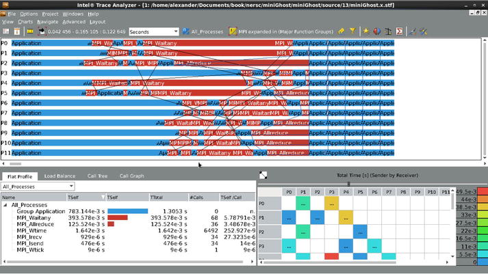
Figure 5-16. Typical MiniGhost exchange pattern (Workstation, 12 MPI processes, 4 OpenMP threads)
This patch corresponds to the very first and most expensive exchange during the program execution. Rather small per se, it becomes a burden due to endless replication; all smaller MPI communication segments after this one follow the same pattern or at least have a pretty imbalanced MPI_Allreduce inside (not shown). It is clear that the first order of the day is to understand why the MPI_Waitany has to work in such irregular circumstances, and then try to correct this. It is also possible that the MPI_Allreduce will recover its dignity when acting in a better environment.
By the looks of it, the pattern in Figure 5-16 resembles a typical neighbor exchange implemented by nonblocking MPI calls. Since the very first MPI_Allreduce is a representative one, we have no problem identifying where the prior nonblocking exchange comes from: a bit of source code and log file browsing lead us to the file called MG_UNPACK_BSPMA.F, where the waiting is done using the MPI_Waitany on all MPI_Request items filled by the prior calls to MPI_Isend and MPI_Irecv that indeed represent a neighbor data exchange. In addition to this, as the name of the file suggests and the code review confirms, the data is packed and unpacked using the respective MPI calls. From this, at least three optimization ideas of different complexity emerge:
- Relatively easy: Use the MPI_Waitall or MPI_Waitsome instead of the fussy MPI_Waitany. The former might be able to complete all or at least more than one request per invocation, and do this in the most appropriate order defined by the MPI implementation. However, there is some internal application statistics collection that is geared toward the use of MPI_Waitany, so more than just a replacement of one call may be necessary technically.
- Relatively hard: Try to replace the nonblocking exchange with the properly ordered blocking MPI_Sendrecv pairs. A code review shows that the exchanges are aligned along the three spatial dimensions, so that a more regular messaging order might actually help smoothe the data flow and reduce the observed level of irregularity. If this sounds too hard, even making sure that all MPI_Irecv are posted shortly before the respective MPI_Isend might be a good first step.
- Probably impossible: Use the MPI derived datatypes instead of the packing/unpacking. Before this deep modification is attempted, it should be verified that packing/unpacking indeed matters.
This coding exercise is only sensible once the MPI_Allreduce issue has been dealt with. For that we need to look into the node-level details in the later chapters of this book, and then return to this issue. This is a good example of the back-and-forth transition between optimization levels. Remember that once you introduce any change, you will have to redo the measurements and verify that the change was indeed beneficial. After that is done, you can repeat this cycle or proceed to the node optimization level we will consider in the following chapters, once we’ve covered more about advanced MPI analysis techniques (to be continued in Chapter 6).
EXERCISE 5-13
Investigate the miniGhost MPI_Init overhead and clarify whether this is a Heisenbug or not. If it is, contact Intel Premier and report the matter.
EXERCISE 5-14
Return here once the MPI_Allreduce load imbalance has been dealt with, and implement one of the proposed source code optimizations. Gauge its effect on the miniGhost benchmark, especially at scale. Was it worth the trouble?
Using Advanced Analysis Techniques
We have barely scratched the surface of capabilities offered by the Intel MPI and Intel Trace Analyzer and Collector. This section introduces more advanced features that you may need in your work, but you will have to read more about them before you can start to use them.
Automatically Checking MPI Program Correctness
We started with the premise of a correctly written parallel application. Here’s the truth, though: there are none. That is, there are some applications that manifest no apparent errors at the moment. Even as we were writing this book, we detected several errors in candidate programs of various levels of maturity, from our own naïve code snippets to the venerable, internationally recognized, and widely used benchmarks. Some programs would not build, some would not run, some would break on ostensibly valid input data, and so on. This is all a fact of life.
Fortunately, if you use Intel MPI and ITAC, you can mitigate at least some of the risk in trying to optimize an erroneous program. Just add option -check_mpi to your application build string or the mpirun, run string, and the ITAC correctness checking library will start watching all MPI transfers and checking them for many issues, including incorrect parameters, potential or real deadlocks, race conditions, data corruption, and more.
This may cost quite some a bit at runtime, especially if you ask for the buffer check sums to be computed and verified, or you used the valgrind in addition to check the memory access patterns. However, in return you will get at least some of that warm and fuzzy feeling that is otherwise unknown to programmers in general and to parallel programmers in particular; that feeling, though, is the almost certain yet dangerously wrong belief that your program is MPI bug free.
Comparing Application Traces
You have seen how we compared real and ideal traces (see Figure 5-12). Actually, this is a generic feature you can apply to any two traces. While comparing two unrelated traces might be a bit off topic, comparing two closely related traces may reveal interesting things. For example, you can compare two different runs of the same application, done on different process counts or just having substantially different performance characteristics on the same process count. Looking into the traces side by side will help you spot where they differ. This is how to go about it:
- Easiest of all, open two trace files you want to compare in one ITAC session when starting up. This is how you can do this:
$ traceanalyzer trace1.stf trace2.stf - If you are already in an ITAC session where you have been analyzing a certain trace file, open another file via the global File/Open menu, and then use the File/Compare item.
- If you want to do this by hand, open the files in any way described above, configure to your liking the charts you want to compare, and then use the global View/Arrange menu item to put them side by side or on top of each other.
For example, if you do any of this for the real and ideal files illustrated in Figure 5-12, you will get the results shown in Figure 5-17.
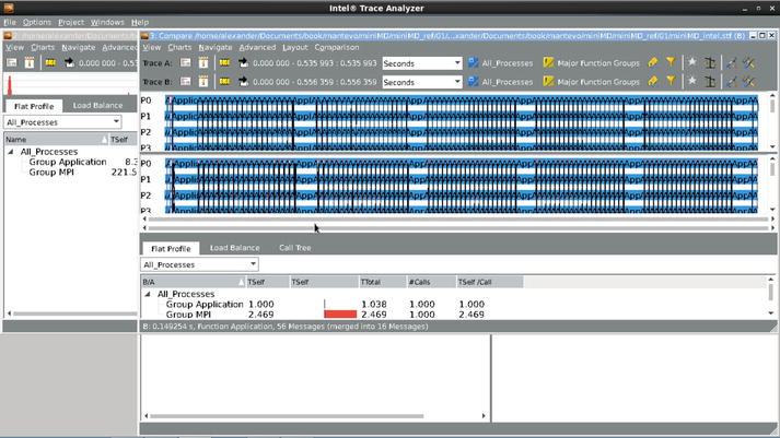
Figure 5-17. MiniMD real and ideal traces compared side by side (Workstation, 16 MPI processes)
This view confirms the earlier observation that, although there may be up to 2.5 times improvement to haul in the MPI area, the overall effect on the total program’s execution time will be marginal. Another interesting view to observe is the Breakdown Mode in the imbalance diagram shown in Figure 5-18 (here we again changed the default colors to roughly match those in the event timeline).

Figure 5-18. MiniMD trace file in ITAC imbalance diagra breakdown mode (Workstation, 16 MPI processes)
From this view you can conclude that MPI_Wait is probably the call to investigate as far as pure MPI performance is concerned. The rest of the overhead comes from the load imbalance. If you want to learn more about comparing trace files, follow up with the aforementioned serialization tutorial.
Instrumenting Application Code
Once in a while you may want to know exactly what is happening in the user part of the application, rather than just observe the blue Group Application mentioned in the respective ITAC charts. In this case you can use several features provided by Intel tools to get this information:
- Probably the easiest is to ask Intel compiler do the job for you. Add the compiler option -tcollect to get all source code functions instrumented to leave a trace in the ITAC trace file. This option needs to be used both at the compilation and at the linkage steps. If the number of the resulting call tracing events is too high, use the -tcollect-filter variety to limit their scope. You may—and probably should—apply these features selectively to those files that interest you most; otherwise, the trace file size may explode. You can find more details in the ITC documentation.26
- If you want complete control and are willing to invest some time, use the ITAC instrumenting interface described in the documentation mentioned above. An instrumentation source code example that comes with the ITAC distribution will be a good starting point here.
You can learn more about these advanced topics and also control the size of the trace file, the latter which is very important if you want to analyze a long running or a highly scalable application, in the Tutorial: Reducing Trace File Size.27
Correlating MPI and Hardware Events
As a final point before we close the MPI optimization, we give a recommendation on how to correlate the ITAC trace events with the hardware events, including those registered by the Intel VTune Amplifier XE data collection infrastructure.28 As usual, there is more than one way to do this.
Collecting and Analyzing Hardware Counter Information in ITAC
Believe it or not, you can collect and display a lot of hardware counter information right in the ITAC. Its facilities are not as extensive and automated as those of VTune Amplifier XE; however, they can give you a good first hack at the problem. You can read about this topic in the ITAC documentation. Note that quite a bit of hacking will be required upfront.
Collecting and Analyzing Hardware Counter Information in VTune
If you have no time for hacking, you can choose the normal way. First, you need to launch VTune Amplifier XE. There are, again, several methods to do so:
- Launch amplxe-cl with mpirun. For example: Collect 1 result/rank/node from M nodes – M result directories in total:
$ mpirun <machine file> -np <N> ... amplxe-cl -collect <analysis type> ./your_appAssumptions: N>M and at least 1 rank/node.
- Collect 2 hotspots on the host ‘hostname’:
$ mpirun -host 'hostname' -np 14 ./a.out :
         -host 'hostname' -np 2 amplxe-cl –r foo -c hotspots
./your_app - Launch mpirun with amplxe-cl. For example: Collect N ranks in one result file on a node (e.g., ‘hostname’):
$ amplxe-cl -collect <analysis type> ... -- mpirun -host ‘hostname’ -np <N> ./your_app
Limitation: Currently collects only on the localhost.
We will cover the rest of this topic in Chapter 6, but you may want to read the Tutorial: Analyzing MPI Application with Intel Trace Analyzer and Intel VTune Amplifier XE as well.29
Summary
We presented MPI optimization methodology in this chapter in its application to the Intel MPI Library and Intel Trace Analyzer. However, you can easily reuse this procedure with other tools of your choice.
It is (not so) surprising that the literature on MPI optimization in particular is rather scarce. This was one of our primary reasons for writing this book. To get the most out of it, you need to know quite a bit about the MPI programming. There is probably no better way to get started than by reading the classic Using MPI by Bill Gropp, Ewing Lusk, and Anthony Skjellum30 and Using MPI-2 by William Gropp, Ewing Lusk, and Rajeev Thakur.31 If you want to learn more about the Intel Xeon Phi platform, you may want to read Intel Xeon Phi Coprocessor High-Performance Programming by Jim Jeffers and James Reinders that we mentioned earlier. Ultimately, nothing will replace reading the MPI standard, asking questions in the respective mailing lists, and getting your hands dirty.
We cannot recommend any specific book on the parallel algorithms because they are quite dependent on the domain area you are going to explore. Most likely, you know all the most important publications and periodicals in that area anyway. Just keep an eye on them; algorithms rule this realm.
References
1. MPI Forum, “MPI Documents,” www.mpi-forum.org/docs/docs.html.
2. H. Bockhorst and M. Lubin, “Performance Analysis of a Poisson Solver Using Intel VTune Amplifier XE and Intel Trace Analyzer and Collector,” to be published in TBD.
3. Intel Corporation, “Intel MPI Benchmarks,” http://software.intel.com/en-us/articles/intel-mpi-benchmarks/.
4. Intel Corporation, “Intel(R) Premier Support,” www.intel.com/software/products/support.
5. D. Akin, “Akin’s Laws of Spacecraft Design,” http://spacecraft.ssl.umd.edu/old_site/academics/akins_laws.html.
6. A. Petitet, R. C. Whaley, J. Dongarra, and A. Cleary, “HPL - A Portable Implementation of the High-Performance Linpack Benchmark for Distributed-Memory Computers,” www.netlib.org/benchmark/hpl/.
7. Intel Corporation, “Intel Math Kernel Library – LINPACK Download,” http://software.intel.com/en-us/articles/intel-math-kernel-library-linpack-download.
8. A. Petitet, R. C. Whaley, J. Dongarra, and A. Cleary, “HPL FAQs,” www.netlib.org/benchmark/hpl/faqs.html.
9. “BLAS (Basic Linear Algebra Subprograms),” www.netlib.org/blas/.
10. Sandia National Laboratory, “HPCG - Home,” https://software.sandia.gov/hpcg/.
11. “Home of the Mantevo project,” http://mantevo.org/.
12. Intel Corporation, “Configuring Intel Trace Collector,” https://software.intel.com/de-de/node/508066.
13. Sandia National Laboratory, “LAMMPS Molecular Dynamics Simulator,” http://lammps.sandia.gov/.
14. Ohio State University, “OSU Micro-Benchmarks,” http://mvapich.cse.ohio-state.edu/benchmarks/.
15. Intel Corporation, “Intel MPI Library - Documentation,” https://software.intel.com/en-us/articles/intel-mpi-library-documentation.
16. J. Jeffers and J. Reinders, Intel Xeon Phi Coprocessor High-Performance Programming (Waltham, MA: Morgan Kaufman Publ. Inc., 2013).
17. “MiniGhost,” www.nersc.gov/users/computational-systems/nersc-8-system-cori/nersc-8-procurement/trinity-nersc-8-rfp/nersc-8-trinity-benchmarks/minighost/.
18. Intel Corporation, “Tutorial: MPI Tuner for Intel MPI Library for Linux OS,” https://software.intel.com/en-us/mpi-tuner-tutorial-lin-5.0-pdf.
19. M. Chuvelev, “Collective Algorithm Models,” Intel Corporation, Internal technical report, 2013.
20. Intel Corporation, “Tutorial: Detecting and Removing Unnecessary Serialization,” https://software.intel.com/en-us/itac_9.0_serialization_pdf.
21. A. Supalov and A. Yalozo, “20 Years of the MPI Standard: Now With a Common Application Binary Interface,” The Parallel Universe 18, no. 1 (2014): 28–32.
22. M. Brinskiy, A. Supalov, M. Chuvelev, and E. Leksikov, “Mastering Performance Challenges with the New MPI-3 Standard,” The Parallel Universe 18, no. 1 (2014): 33–40.
23. “PanFS Storage Operating System,” www.panasas.com/products/panfs.
24. “Parallel Virtual File System, Version 2,” www.pvfs.org/.
25. “Lustre - OpenSFS,” http://lustre.opensfs.org/.
26. Intel Corporation, “Intel Trace Analyzer and Collector - Documentation,” https://software.intel.com/en-us/articles/intel-trace-analyzer-and-collector-documentation.
27. Intel Corporation, “Tutorial: Reducing Trace File Size,” https://software.intel.com/en-us/itac_9.0_reducing_trace_pdf.
28. Intel Corporation, “Intel VTune Amplifier XE 2013,” https://software.intel.com/en-us/intel-vtune-amplifier-xe.
29. Intel Corporation, “Tutorial: Analyzing MPI Application with Intel Trace Analyzer and Intel VTune Amplifier XE,” https://software.intel.com/en-us/itac_9.0_analyzing_app_pdf.
30. W. Gropp, E. L. Lusk, and A. Skjellum, Using MPI: Portable Parallel Programming with the Message Passing Interface, 2nd. ed. (Cambridge, MA: MIT Press, 1999).
31. W. Gropp, E. L. Lusk, and R. Thakur, Using MPI-2: Advanced Features of the Message Passing Interface (Cambridge, MA: MIT Press, 1999).