
![]()
Addressing System Bottlenecks
We start with a bold statement: every application has a bottleneck. By that, we mean that there is always something that limits performance of a given application in a system. Even if the application is well optimized and it may seem that no additional improvements are possible by tuning it on the other levels, it still has a bottleneck, and that bottleneck is in the system the program runs on. The tuning starts and ends at the system level.
When you improve your application performance to take advantage of all the features provided in the hardware, you use all available concurrency, and the application’s execution approaches peak performance, but that peak performance will limit how fast the program can run. A trivial solution to improve performance in such cases is to buy a new and better piece of hardware. But to make an informed selection of new hardware, you would need to find a specific system-level bottleneck that restricts the application performance.
This chapter starts with discussion of the typical system-level tweaks and checks that one can implement before considering purchasing new hardware. These need to be seen as sanity checks of the available hardware before you invest in tuning of your applications on the other levels. The following chapters describe the tools and techniques for application optimization, yet the optimization work in the application must rely on a clean and sane system. This chapter covers what can be wrong with the system and how to find out if that specific system limitation is impacting your application performance.
Classifying System-Level Bottlenecks
System-level bottlenecks, or issues that do not allow reaching hardware peak performance, arise from limitations in either hardware or software components that are generally outside user and application control. The reality is that any computer system has hardware performance limitations. In most cases, the difference between a “good” and a “bad” system is only one thing: whether its limitations cause your application to be slow. The application developer can avoid some performance impact brought about by system bottlenecks, but generally it requires a system administrator to debug and reconfigure the system. But before an application developer or a user can produce claims to the system administrator, the bottleneck has to be identified and its impact characterized and quantified.
The root causes of system bottlenecks can be split into two major categories, depending on their origin:
- Condition and the run-time environment
- Configuration of hardware, firmware, or software
The first may be present temporarily, appear from time to time, and may go away and come back unless the issues are identified and fixed. The second includes issues that are really static in time unless the system is reconfigured, and they are caused by limitations in how the system was built (for instance, component selection, their assembly, and their configuration).
Identifying Issues Related to System Condition
Performance problems caused by the system condition or the environment where it operates are probably the hardest to diagnose, so let’s start with them. The main cause of these system bottlenecks are the conditions under which the application executes or makes the transient changes to its runtime environment. Some specific examples include the following:
- Shared resource conflicts: A program running on a shared cluster may get fewer resources, depending on other applications executed on other nodes of the cluster at the same time. Two major shared resources in an HPC cluster are the shared parallel file system and the interconnect between the cluster nodes. Sometimes there can be memory-related bottlenecks when some cluster nodes are shared by different jobs, which may cause conflicts between these jobs depending on the specific scheduling.
- Throttling: Processors and memory modules in the cluster nodes may experience performance throttling caused by overheating or power delivery limitations. This is usually a data center–level issue, and there is really nothing an application developer can do: the system administrators and the vendor of the cluster have to revise their cooling or power delivery subsystem configurations.
- Faults: It may be a rather rare case, but if something in the hardware or software starts failing, it may temporally impact performance. A fault does not necessarily lead to system or application crash. Modern hardware has very sophisticated resiliency and error-correction mechanisms, and it is often able to recover from many types of errors, such as a single-bit data corruption in the memory or loss of a packet in transit. While these recovery mechanisms enable programs to continue running despite the faults occurring, they do take time for their work and may produce significant performance overhead for the user application running on the system.
Usually, detection and repair of the system-level issues is a responsibility of system administrators and the system provider. We do recommend that administrators ask vendors about Intel Cluster Ready certification for their systems. The certified cluster comes with a software tool from Intel, called the Intel Cluster Checker, and it’s a key element of the Intel Cluster Ready validation process. The tool helps verify that cluster components are working when the cluster is being deployed and also that the components continue working together as expected throughout the cluster lifecycle. However, sometimes users need to raise awareness of observed performance problems before the issue is investigated.
There are several things you can do during development of an application or while setting up a job scripts that can help debug condition-related problems:
- Check shared resource conflicts by timing your code: Insert a collection of timings into your application to gather execution time for the known long-lasting activities that depend on shared resources.
- For instance, if your application reads from or writes to a shared parallel file system, it may be beneficial to determine the time spent on the input/output (I/O) operations and report this time in the program output.
- For MPI applications, you may measure the time when there are known large message-passing operations, or routinely gather MPI time statistics produced by Intel MPI library (as discussed in Chapter 5). If in certain application runs the I/O or MPI take more time than usual, it may indicate a conflict over these shared resources or a fault in the file system (for instance, a failing disk, which may cause RAID rebuild with subsequent slowdown of I/O operations) or in the network fabric (for example, a broken cable, which may cause sporadic packet loss resulting in multiple attempts to deliver the respective messages).
- Count thermal and power throttling events. Unfortunately, quite often an observed class of system-level issues is caused by throttling problems. But it is very easy to check if any thermal or power throttling occurred on any server, even if you do not have the administrative privileges. The Linux operating system kernel provides relevant counters for events such as the processor overheating or excessive power use. The script presented in Listing 4-1, here named check_throttle.sh (works for Bash compatible shells on Linux), will let you know how many throttling events have occurred since the last booting of the operating system.
Listing 4-1. Contents of check_throttle.sh Script to Count Throttling Events
#!/bin/sh
let CPU_power_limit_count=0
let CPU_throttle_count=0
for cpu in $(ls -d /sys/devices/system/cpu/cpu[0-9]*); do
  if [ -f $cpu/thermal_throttle/package_power_limit_count]; then
  let CPU_power_limit_count+=$(cat $cpu/thermal_throttle/
  package_power_limit_count)
  fi
  if [ -f $cpu/thermal_throttle/package_throttle_count]; then
    let CPU_throttle_count+=$(cat $cpu/thermal_throttle/package_
     throttle_count)
  fi
done
echo CPU power limit events: $CPU_power_limit_count
echo CPU thermal throlling events: $CPU_throttle_count
The expected good values for both printed lines should be zero, as shown in Listing 4-2.
Listing 4-2. Example of check_throttle.sh Script Run and Output
$ ./check_throttle.sh
CPU power limit events: 0
CPU thermal throlling events: 0
Anything other than zero indicates the presence of throttling events, which usually impacts performance significantly. During the throttling events, the clock frequency of the processors is reduced to save power, relying on the fact that the active power has a cubic dependency upon the voltage/frequency. Another technology to mitigate overheating of the chip is to insert duty cycles (when the processor clock is not running). This helps in reducing the processor temperature if a critical temperature is reached, but it significantly hurts performance of the applications.
- Check for failure events. Some of the more advanced techniques for detecting system-level issues may require root privileges, and thus can only be used by the system administrators. Programs such as mcelog1 for Linux decode machine check events on modern Intel Architecture machines running a Linux OS with 64-bit kernel. Machine checks can indicate failing hardware, system overheats, bad memory modules, or other problems. If the tool is run regularly, it is useful for predicting server hardware failures before an actual server crash or there’s appearance of visible performance impact on user applications.
- Ensure interconnect fabrics and storage are clean. Additional areas of responsibility for the system administrators and vendors are to ensure the interconnect fabric is clean and the storage is built properly. This means that there are no bad cables, no bad ports, and no bad connectivity in the interconnection network, and that the storage arrays are complete, and are built and operated correctly.
Characterizing Problems Caused by System Configuration
The other class of issues listed above can be caused by the configuration of hardware or software that the application is run on. This is also generally outside system user control, and administrative privileges are required to alter the system settings. However, the user can check some of these settings, and may alert system administrators if any important misconfigurations are observed. For instance:
- Check that the system software and the operating system (OS) versions are the latest. The OS has to be relatively new to support all important hardware features, specifically in the platforms and in the processors. As a rule of thumb (applied largely to Linux distributions), if the OS was released more than a year before the processor of the server, it likely should be updated or at least a newer kernel and major system libraries should be installed. The new processor and platform generations bring new features that almost always need proper support by the OS. Some of these features are the instruction set extensions brought out by Intel almost every year, and the changes in the mainstream server platform technologies instituted about every two years. Lack of support for the new features will not make the old OS dysfunctional; backwards compatibility normally allows old operating systems to boot and work, although inefficiencies will likely be observed.
- Review OS configuration. A good OS for HPC systems has to be nondisturbing to the applications. In the HPC world (unlike some enterprise computing areas), a single user application usually exclusively owns the execution resources of several computational nodes, so the presence of any other activity on these nodes is undesirable, for this generates random interruptions of computations that may negatively impact a parallel application’s performance. And it is here that most of the OS configuration issues are observed nowadays. Unfortunately, no universal checklists exist for all possible disturbing factors because there is a wide variety of Linux distributions and site-specific packages that are still necessary on cluster compute nodes. However, there is one tool we recommend to the system administrators for analysis of the OS disturbance: PowerTOP.2 It was originally developed by the Intel Open Source Technology Center to help identify power-hungry applications causing OS wakeups in mobile and embedded platforms. At the same time it is a great tool for reducing OS wakeups and to experiment with the various power management settings for cases where the Linux distribution has not enabled these settings by default. The interactive mode of PowerTOP helps to quickly reveal disturbing activities without expending great effort. We can run PowerTOP on our development workstation with CentOS 6.5, like this:
$ sudo powertop Note Here, prior to running the powertop command, we used another command: sudo. This addition instructs the operating system to use administrator or superuser privileges to execute the following command, while not asking for the super user password. In order to be able to use sudo, the system administrator has to delegate the appropriate permission to you—usually by means of including you in a specific group (such as wheel or adm) and editing system configuration file /etc/sudoers. Depending on the configuration, you may be asked to enter your password.
The output of running PowerTOP presented in Figure 4-1 shows that the OS wakeups disturbing other applications happen over 50 times per second and that the two most disturbing residents in the OS are the kipmi0 kernel process and the alsa device driver for the sound system. Impact from kipmi0 is rather large: the processing time takes 998 milliseconds every second—less than 2 milliseconds short of an entire second—thus taking away one complete core from the user applications.
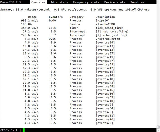
Figure 4-1. PowerTOP run in interactive mode
The alsa driver is the one for the sound system, which is not usually used in HPC systems and can safely be removed. In general, it is good practice to remove all unused software that by default may be installed with your favorite OS distribution (for instance, the mail servers, such as sendmail, or the Bluetooth subsystem that are not generally needed in HPC cluster compute nodes), and thus should either be uninstalled from the OS or be disabled from the startup process.
The kipmi0 is part of the OS kernel that is responsible for the work of the intelligent platform management interface (IPMI) subsystem,3 which is often used to monitor various platform sensors, such as those for the CPU temperature and voltage. This may be required by the in-band monitoring agents of the monitoring tools like lm_sensors,4 Ganglia,5 or Nagios.6 Although kipmid is supposed to use only the idle cycles, it does wake up the system and can affect application performance. The good news is that it is possible to limit the time taken by this kernel module by either adding the line options ipmi_si kipmid_max_busy_us=1 to the ipmi.conf file under /etc/modprobe.d/, or by executing the following command:
$ sudo bash -c
'echo 1 > /sys/module/ipmi_si/parameters/kipmid_max_busy_us'
This will limit the kipmid CPU time and the number of times it wakes up the OS.
After these two changes to the OS configuration, the number of wakeups per second on our test system was reduced and, more important, CPU usage went down. The CPU usage in the OS’s idle state is around 1.5 percent (where at least 1 percent is taken by the PowerTOP itself), and the processor usage by the kipmi0 is reduced to around 1 ms per second. The next biggest cause of OS wakeups is the timer process that takes only a third of a millisecond every second.
Other configurations or versions of operating systems may have a very different set of hardware and software components, but using tools like Linux top and the PowerTOP will help you identify the time-consumers and serve as a guide to improving system idle-state overhead.
- Check BIOS settings: As the next step after OS improvement, it is worth checking important parameters of the basic input/output system (BIOS). Unlike BIOS setups in client platforms, BIOS in a server provides a lot more options to tune the system characteristics for different application workloads. While the available choice of settings is a very good way to support multiple different usages of the server platforms, it may also lead to inefficient settings for your specific applications. And although the OEMs delivering high-performance computing solutions try to configure their servers in a proper way, it may still be good to follow some basic recommendations for several important BIOS settings.
The BIOS provides a summary of detected hardware: processor type and speed, memory capacity, and frequency. For instance, if there is a memory module failure, it will not be detected and presented by the BIOS to the operating system, and the server will boot. And if the memory module failure is not noticed, the system will continue working, but the memory capacity and performance will be lower than expected.
- As the HPC applications performance is very often dependent on the memory subsystem performance, the settings affecting the main memory are among the most important to study. One of these settings is the “NUMA mode” selection. In multi-socket platforms with the memory controllers integrated into the processor running a modern OS, enabling the NUMA support presents the physical memory of the system as a split between the local and remote to each socket (as shown inListing 2-1 in Chapter 2). Efficient use of NUMA requires software optimizations that we discuss in greater detail in Chapter 6.
- The status of power management technologies and power/performance settings (such as Intel Enhanced SpeedStep Technology, EIST, and Intel Turbo Mode) are available in the BIOS setup to shift the balance between energy draw and performance: reducing the power draw may negatively affect the application’s speed.
- Another source of configuration issues may lay in excessive use of the resiliency technologies built into the memory subsystem. In order to increase server uptime and prevent crashes from memory failures, it is possible to configure so-called memory mirroring, sparing, or lockstep operations. These technologies help increase server availability, but they come at a cost to memory capacity and performance, sometimes impacting memory bandwidth by a factor of 2.
![]() Note For the best possible performance, check that the memory is configured in the channel interleave or the independent mode the BIOS.
Note For the best possible performance, check that the memory is configured in the channel interleave or the independent mode the BIOS.
Understanding System-Level Performance Limits
Practically, the best way to identify system-level issues is to check the major system parameters with simple yet powerful kernel tests. These tests usually do not take a lot of time to set up and run, and they are an essential part of the acceptance process when a supercomputer is handed over from the vendor to the customer. Moreover, periodic runs of these tests may reveal system health issues during its day-to-day operation. As the HPC software paradigm to a large extent relies on a high-performing cluster of uniform (in configuration and performance) computational nodes, running these tests on every node of the cluster will help to ensure performance uniformity across all similarly configured components in the HPC system.
We distinguish several important subsystems that the kernel benchmarks should focus on:
- Compute subsystem: The main processors and coprocessors that can be installed in every cluster node.
- Main memory subsystem: Test the main memory performance characteristics. When Intel Xeon Phi coprocessors are installed, the GDDR5 memory of the coprocessor card needs to be tested in similar way as the main memory.
- Cluster interconnect network: Used to wire the computational nodes together and to access the high-performance storage subsystem.
Each subsystem can be tested separately, and the performance results can be compared to expected good values from the vendor datasheets, as well as between different cluster nodes. There are large numbers of application kernels that can be designed to check the efficiency of different subsystems. Here we review those that have proved to be useful in practice.
Checking General Compute Subsystem Performance
One of the widely used stress tests in HPC is the High Performance Linpack (HPL) benchmark. It is the benchmark used to rank supercomputers in the TOP500 list published at www.top500.org twice a year. Despite this, the relevance of the HPL to real HPC applications is debated. However, it can certainly be used to validate the system performance and stability. There are many reference results for different architectures found on the TOP500 list, which gives a baseline for comparison with your results. (In the following chapters we will also use HPL a couple of times for demonstration purposes.)
The main disadvantage of the HPL benchmark is that it may be hard to set up and find optimal parameters, so bad performance may be not an indication of a slow node or cluster but, rather, be the result of poor benchmark configuration. Also with HPL, it would be hard to identify a slow node in a cluster—in case one exists. This is why Intel engineers not only ship an optimized version of the HPL benchmark along with the Intel Math Kernel Library (MKL) but also provide a small program to test compute nodes performance called nodeperf.c. This is a simple MPI program that runs a highly optimized version of a double precision general matrix multiply (DGEMM) library routine from the MKL. This routine is also the core of the HPL test. As the MKL provides optimized versions of DGEMM and many other widely used routines, you can be sure that the test will be optimized for the latest Intel microprocessors.
Let’s see how to check the uniformity and performance of an eight-node cluster using the nodeperf tool. First, you may need to load the environment variables for the Intel software tools to be used shortly. The first line will load the compiler environment settings into the Bash shell, and the second will set up variables for the Intel MPI library:
$ source /opt/intel/composerxe/bin/compilervars.sh intel64
$ source /opt/intel/impi_latest/intel64/bin/mpivars.sh
You will find the scripts for the C-shell under the same folder as the scripts for the Bash-compatible shells. The source code of the nodeperf application can be found in the source folder of the HPL benchmark that comes with the Intel MKL. If Intel Parallel Studio XE 2015 Cluster Edition is installed into its default folder, you can copy the nodeperf.c source file to your current directory, where the benchmark will be compiled and later executed (it is expected that this directory is shared among all cluster nodes):
$ cp $MKLROOT/benchmarks/mp_linpack/nodeperf.c ./
Compile the nodeperf program using the Intel MPI compile wrapper script for Intel compiler with the optimizations enabled to at least -O2 level, tuning for the instruction set supported on the build machine (either by using the -xHost or by directly specifying another instruction set target as described in Table 1-1), enabling OpenMP support (-qopenmp), and linking with the MKL library for the optimized version of the DGEMM routine (-mkl):
$ mpiicc -O2 -xHost -qopenmp -mkl nodeperf.c -o nodeperf
Successful completion of the command should produce an executable binary nodeperf in the current working directory. It is ready to run. Just before the run, however, you need to set a few important environment variables that control the number of OpenMP threads and their placement on the system:
$ export OMP_NUM_THREADS=24
$ export OMP_PLACES=cores
The first command requests 24 OpenMP threads. This is equal to the number of physical processor cores in every node of our cluster: each of two CPUs has 12 cores, so we ask exactly one thread per physical core. In case OMP_NUM_THREADS is not explicitly set up, the Open MP runtime library will use all processors visible to the OS, which, in the case of enabled Hyper Threading, will lead to assignment of two Open MP threads to each physical core. The OMP_PLACES environment variable instructs Intel OpenMP runtime to distribute threads between the cores in the system, so that two different threads will not run on one physical core. Now we’re ready to start the test using the mpirun command that requests eight ranks (using the -np 8 option), with only one rank per node (-ppn 1):
$ mpirun -np 8 -ppn 1 -hosts esg003,esg004,esg005,esg006,esg007,esg008,esg00
9,esg010 ./nodeperf
![]() Note The -hosts option for the mpirun command explicitly lists the names of hosts allocated for our job by the scheduler, and we provide it here for illustration purposes. More convenient is to provide the list of hosts the program will run on in a separate file; or in a majority of cases, Intel MPI can pick it up automatically from the resource manager of the job scheduling system. Please consult your cluster documentation to see how the MPI jobs are to be run on your cluster.
Note The -hosts option for the mpirun command explicitly lists the names of hosts allocated for our job by the scheduler, and we provide it here for illustration purposes. More convenient is to provide the list of hosts the program will run on in a separate file; or in a majority of cases, Intel MPI can pick it up automatically from the resource manager of the job scheduling system. Please consult your cluster documentation to see how the MPI jobs are to be run on your cluster.
The output of nodeperf run is shown in Listing 4-3.
Listing 4-3. Example Output of nodeperf (Cluster, 8 Nodes)
Multi-threaded MPI detected

The time/date of the run... at Mon May 12 06:11:29 2014

This driver was compiled with:
        -DITER=4 -DLINUX -DNOACCUR -DPREC=double
Malloc done. Used 827090096 bytes
(0 of 8): NN lda=10000 ldb= 168 ldc=10000 0 0 0 519260.972 esg003
(1 of 8): NN lda=10000 ldb= 168 ldc=10000 0 0 0 506726.008 esg004
(2 of 8): NN lda=10000 ldb= 168 ldc=10000 0 0 0 517275.263 esg005
(3 of 8): NN lda=10000 ldb= 168 ldc=10000 0 0 0 519160.998 esg006
(4 of 8): NN lda=10000 ldb= 168 ldc=10000 0 0 0 512007.115 esg007
(5 of 8): NN lda=10000 ldb= 168 ldc=10000 0 0 0 513921.217 esg008
(6 of 8): NN lda=10000 ldb= 168 ldc=10000 0 0 0 530959.117 esg009
(7 of 8): NN lda=10000 ldb= 168 ldc=10000 0 0 0 515852.598 esg010
The last two columns present the achieved performance of the DGEMM routine in MFLOPS and the respective host name where the nodeperf was run. We immediately find that node esg004 is the slowest one and esg009 is the fastest, and the performance difference between the fastest and the slowest nodes is about 4.8 percent.
EXERCISE 4-1
Taking into account that our computational nodes are built using two Intel Xeon E5-2697 v2 processors (each with 12 cores and 2700 MHz nominal clock frequency), with support of the Intel AVX instruction set (so each core is capable of delivering up to 8 Flops/cycle in double precision), compare the performance achieved on every node as a ratio between the achieved performance and the peak performance.
After completing Exercise 4-1, you should have found that three nodes demonstrate performance higher than the theoretical peak. How is this possible? This happens because the peak performance was calculated using the nominal rated frequency of the processor (2.7 GHz). But by default, Intel Turbo Boost technology is enabled. This allows for processors running at a higher frequency than the nominal one when the CPU power consumption stays within the specification and the cooling system can cool the processor package below its critical temperature. An Intel Xeon E5-2697 v2 processor can run at a up to 300 MHz higher clock speed in the Turbo Boost, thus reaching up to 3 GHz. When Turbo Boost is disabled in BIOS settings, though, the processor clock frequency cannot exceed the nominal 2.7 GHz, and consequently the performance reported by nodeperf is lower, while still above 90 percent from the peak performance, as shown in Listing 4-4.
Listing 4-4. Output of nodeperf with Turbo Boost Disabled (Cluster, 8 Nodes)
Multi-threaded MPI detected

The time/date of the run... at Mon May 12 06:25:39 2014

This driver was compiled with:
        -DITER=4 -DLINUX -DNOACCUR -DPREC=double
Malloc done. Used 827090096 bytes
(0 of 8): NN lda=10000 ldb= 168 ldc=10000 0 0 0 482853.191 esg003
(1 of 8): NN lda=10000 ldb= 168 ldc=10000 0 0 0 469475.454 esg004
(2 of 8): NN lda=10000 ldb= 168 ldc=10000 0 0 0 469658.038 esg005
(3 of 8): NN lda=10000 ldb= 168 ldc=10000 0 0 0 480475.968 esg006
(4 of 8): NN lda=10000 ldb= 168 ldc=10000 0 0 0 469907.603 esg007
(5 of 8): NN lda=10000 ldb= 168 ldc=10000 0 0 0 479765.330 esg008
(6 of 8): NN lda=10000 ldb= 168 ldc=10000 0 0 0 480635.807 esg009
(7 of 8): NN lda=10000 ldb= 168 ldc=10000 0 0 0 469960.729 esg010
One final observation: this result also shows that the performance difference between the fastest and the slowest nodes in the cluster is only 2.8 percent and is lower than the case when the Turbo Boost is enabled. Turbo Boost can help achieve better performance results; however, the observed performance variations between the nodes will be higher, depending on each node,s conditions.
Testing Memory Subsystem Performance
Memory subsystem performance can be quickly characterized by measuring the main memory bandwidth and the latency, and comparing results to the good expected values and the values for different cluster nodes.
- Characterizing memory bandwidth: The most famous test to check the memory bandwidth is the STREAM benchmark:7 it is quick, easy to set up, and easy to run. It consists of just one source file that can be downloaded from the official benchmark site. After downloading the source code, you can compile it using the Intel compiler as follows:
$ icc -O3 -xHost -mcmodel=medium -qopenmp stream.c -o streamAlso, before compilation, you may consider increasing the STREAM_ARRAY_SIZE parameter to increase the size of the memory used during the benchmark from the default 0.2 GiB,8 which may be too small to get reproducible results. For instance, setting the STREAM_ARRAY_SIZE to 800000000 elements will cause the benchmark to use 18 GiB of memory. In this case the compiler option -mcmodel=medium is required to remove the restriction of 2 GiB on the size of the arrays.
Out of the entire output of the STREAM benchmark you may pick just the values of the TRIAD component that executes the following computational kernel a(i) = b(i) + q*c(i). For convenience, we have put the stream command and necessary parsing of the results into a shell script with the file name 2run.sh, shown in Listing 4-5. In that script we assume the script with environment variables settings and compiled stream binary reside in the same folder as the 2run.sh script file. To keep the scripts portable, we have also used a dynamic way to calculate the number of physical cores in the server and set OMP_NUM_THREADS variable to that value.
Listing 4-5. Contents of 2run.sh Script to Run STREAM Benchmark and Output TRIAD Result
#/bin/sh
. `dirname $0`/0env.sh
export OMP_NUM_THREADS=$(cat /proc/cpuinfo| awk 'BEGIN{cpus=0}
/processor/{cpus++}
/cpu cores/{cpu_cores=$4}
/siblings/{siblings=$3}
END{print cpus*cpu_cores/siblings}')
export OMP_PLACES=cores
`dirname $0`/stream | awk -v host=$(hostname) '/Triad:/{printf
"%s: %s
",host,$2}'
You can run this script using the following command, assuming the current working directory where the script resides is accessible from all nodes.
$ mpirun -np 8 -ppn 1 ./2run.sh Note In this command, we omitted listing hostnames to run the test on, and depending on your cluster setup, you may or may not have to do it explicitly in the mpirun command.This will produce the output presented in Listing 4-6.
Listing 4-6. Example Output of the STREAM Benchmark (Cluster, 8 Nodes)
esg145: 84845.0
esg215: 85768.2
esg281: 85984.2
esg078: 85965.3
esg150: 85990.6
esg084: 86068.5
esg187: 86006.9
esg171: 85789.7
The measured memory bandwidth around 85 GB/s represents approximately 83 percent of the peak memory bandwidth achieved by a dual-socket platform with quad channel DDR3 memory running at 1600 MHz. The above scores represent very good efficiency. The STREAM TRIAD benchmark should achieve values of 80 to 85 percent from the peak memory bandwidth on Xeon E5 platforms.
- Measuring memory latency: The second component of the memory performance is the memory access latency. Unlike bandwidth, latency is much harder to measure correctly and to get results that make sense.
First, you need to decide on the conditions of the environment in which to measure latency, such as whether idle latency (when no other significant workload is running) or loaded latency is to be measured (when multiple workloads run at the same time). The former is a lot easier to implement, but you may need to make sure that processor cores do not go into a sleep state while measuring the idle latency. The latter will require additional applications executing to stress the memory bus and quantify the intensity of that workload.
- While measuring memory latency you need to ensure the results are really not including the caching effects. The processor caches become larger and more sophisticated with each generation, and the tools must be updated to keep up with the improvements in the cache logic.
- Finally, the more advanced characterization of the system will require a tool measuring not only memory latency but also cache access latency. And considering multi-socket systems, this tool should measure latency for accessing local and remote memory when systems with non-uniform memory architecture (NUMA) are benchmarked.
Several Intel engineers came together to write a memory latency checker tool that is designed to help quantify latency for accessing main memory and caches. Intel Memory Latency Checker9 prints out a matrix of the latencies and bandwidths (for various read:write ratios) when accessing the local and remote memory nodes from all the sockets in a multi-socket system, as shown in Listing 4-7 for a dual-socket system. The advanced usages include options to measure specific configurations, such as cache latencies, loaded latency (to produce charts similar to Figure 2-15), bandwidth matrices, and so on. In order to precisely measure latency and bandwidth, the tool requires access to the processor’s internal performance counters. To gain access to these counters, the tool must be run with root privileges. We achieved that via the sudo command.
Listing 4-7. Example Output of Intel Memory Latency Checker for a Dual-Processor Server
$ sudo ./mlc --latency_matrix

Intel(R) Memory Latency Checker - v2.1
Command line parameters: --latency_matrix

Using buffer size of 200.000MB
Measuring idle latencies (in ns)...
         Memory node
Socket   0       1
     0    69.7   123.7
     1   124.5    70.3
The results of the local and remote memory latencies allow measuring the NUMA factor between the NUMA nodes in the system; for our specific system, this yields a value around 1.77 between sockets 0 and 1 (calculated as the ratio between 123.7 and 69.7, taken from the output inListing 4-7). This quantifies the impact of the wrong memory pinning on the memory access latency, which is specifically important for the OpenMP programs that we will discuss in Chapter 6.
EXERCISE 4-2
Run the STREAM benchmark and Intel Memory Latency Checker on your system to determine maximum achievable memory bandwidth and access latency. What share of the peak memory throughout is achieved on the STREAM test? If your system has NUMA architecture, what NUMA factor does it have?
Testing I/O Subsystem Performance
The input and output (I/O) subsystem deals with everything the computational node has to send to or receive from other computational or storage nodes in the HPC cluster. In many clusters, computational nodes use at least two interconnects: Gigabit Ethernet for general TCP/IP traffic supporting management and monitoring services (for instance, secure shell and Ganglia) and high-speed fabrics, such as InfiniBand, for low-latency and high-bandwidth remote direct memory access (RDMA) traffic of the user applications. Since an InfiniBand link is usually dedicated to the performance-critical data transfers, such as Message Passing Interface (MPI) or access to the parallel file systems, its performance is of main concern. (In Chapter 5 we will cover performance benchmarks using Intel MPI library, and the special suite of tests to validate MPI functions performance: Intel MPI Benchmarks (IMB).) For a basic platform I/O validation, and specifically for understanding if the system delivers expected RDMA performance between two nodes, there are a couple of simple tests available with any InfiniBand installation.
For instance, the software stack coming along with the InfiniBand network drivers usually contains a package called perftest with a set of low-level performance tests. These tests allow for measuring bandwidth and latency for typical RDMA commands, such as
- The read and write operations between two nodes: ib_read_bw, ib_write_bw, ib_read_lat, ib_write_lat,
- The send command and atomic transactions: ib_send_bw, ib_atomic_bw, ib_send_lat, ib_atomic_lat.
The tests require a server to be started on one of the nodes and the client on another. Let’s take two nodes in our cluster (say, esg012 and esg013), and start a server on the node named esg012 as follows:
[esg012]$ ib_read_lat -d mlx4_0
Here, the option -d will request a specific InfiniBand device to be used (alternatively, the tool will select the first device found). The list of available RDMA devices can be obtained using the ibv_devices command, and for our cluster this list looks like this:
$ ibv_devices
    device              node GUID
    ------              ----------------
    scif0               001b68fffe3d7f7a
    mlx4_0              0002c903002f18b0
By providing the mlx4_0 argument in the command, we select that InfiniBand adapter. The same has to be done on client node, esg013, where in addition the hostname of the server should be given. The RDMA read latency test command executed on the client node esg013 and its output are presented in Listing 4-8.
Listing 4-8. Example Output of the RDMA Read Latency Test (Cluster)
[esg013]$ ib_read_lat -d mlx4_0 esg012
----------------------------------------------------------------------------
                    RDMA_Read Latency Test
 Dual-port       : OFF          Device : mlx4_0
 Number of qps   : 1
 Connection type : RC
 TX depth        : 1
 Mtu             : 4096B
 Link type       : IB
 Outstand reads  : 16
 rdma_cm QPs     : OFF
 Data ex. method : Ethernet
----------------------------------------------------------------------------
 local address: LID 0x130 QPN 0x0733 PSN 0xe892fa OUT 0x10 RKey 0x3010939
VAddr 0x00000000f60000
 remote address: LID 0x179 QPN 0x06fe PSN 0x5afd2 OUT 0x10 RKey 0x010933
VAddr 0x000000015c8000
----------------------------------------------------------------------------
 #bytes  #iterations   t_min[usec]    t_max[usec]  t_typical[usec]
 2       1000          1.85           20.96        1.91
----------------------------------------------------------------------------
Here, the measured latency for the 2-bytes messages is equal to 1.91 microseconds. Note that remote direct memory access to a different node takes approximately 15 times longer than access to the memory of the remote socket, and it takes 27 times longer than access to the local memory.
The bandwidth tests are run in a similar way. It may be interesting to see bandwidth for different message sizes, which can be measured by adding the -a command option. Listing 4-9 contains a typical output produced on a client compute nodes for a unidirectional write bandwidth test to the server on the node esg012.
Listing 4-9. Output of the Unidirectional RDMA Read Bandwidth Test (Cluster)
[esg013]$ ib_read_bw -a -d mlx4_0 esg012
---------------------------------------------------------------------------
                    RDMA_Read BW Test
 Dual-port       : OFF          Device : mlx4_0
 Number of qps   : 1
 Connection type : RC
 TX depth        : 128
 CQ Moderation   : 100
 Mtu             : 4096B
 Link type       : IB
 Outstand reads  : 16
 rdma_cm QPs     : OFF
 Data ex. method : Ethernet
----------------------------------------------------------------------------
 local address: LID 0x130 QPN 0x0730 PSN 0x7540e6 OUT 0x10 RKey 0x18010939
VAddr 0x02b15b6bcf000
 remote address: LID 0x179 QPN 0x06fc PSN 0x56dc8e OUT 0x10 RKey 0xf0010932
VAddr 0x02b826895800
----------------------------------------------------------------------------
 #bytes   #iterations  BW peak[MB/sec]    BW average[MB/sec]   MsgRate[Mpps]
      2   1000            8.11               7.82              4.098211
      4   1000           16.56              16.55              4.337238
      8   1000           33.12              33.07              4.334843
     16   1000           66.13              66.07              4.329837
     32   1000          132.47             132.43              4.339469
     64   1000          264.09             254.07              4.162761
    128   1000          517.41             509.61              4.174733
    256   1000         1059.77            1059.05              4.337851
    512   1000         2119.55            2116.35              4.334286
    1024  1000         4205.29            4203.23              4.304106
    2048  1000         5414.21            5410.27              2.770060
    4096  1000         4939.99            4939.20              1.264436
    8192  1000         5251.12            5250.99              0.672127
   16384  1000         5267.51            5267.00              0.337088
   32768  1000         5256.68            5256.65              0.168213
   65536  1000         5263.24            5262.24              0.084196
  131072  1000         5264.72            5262.55              0.042100
  262144  1000         5271.87            5271.63              0.021087
  524288  1000         5272.98            5270.55              0.010541
 1048576  1000         5274.57            5273.48              0.005273
 2097152  1000         5272.47            5271.77              0.002636
 4194304  1000         5271.72            5270.81              0.001318
 8388608  1000         5272.14            5270.38              0.000659
----------------------------------------------------------------------------
Using the default settings for the benchmark, we see that the maximum bandwidth achieved on this test is equal to 5.4 GB/s, which represents approximately 80 percent from the peak bandwidth of the InfiniBand link speed of around 6.8 GB/s.
EXERCISE 4-3
Run the perftest benchmarks on your favorite system to determine the maximum achievable interconnect bandwidth and the latency for RDMA network traffic. What share of the peak network speed is achieved on the bandwidth tests?
Characterizing Application System-Level Issues
System-level bottlenecks determine the performance of well-written and optimized applications. Improving the system characteristics, then, that are in direct relation to the application’s slowest path, such as increasing CPU frequency for a compute bound code, will result in improved performance. But how does one find out what system feature is limiting the application performance? And what is the knowledge this investigation will give us?
The second question is rather easy to answer: finding out that an application is memory bandwidth or I/O bandwidth bound (that is, it spends most of the time transferring data to and from memory or over interconnect) will lead to decisions on how to improve performance. Taking into account Amdahl’s Law and the roofline model discussed in Chapter 2, an understanding of the share of I/O or memory dependent execution time may guide you to a quantitative assessment of potential improvements and provide ideas for improving the algorithms.
Selecting Performance Characterization Tools
Historically, performance issues were qualified as system-level bottlenecks when a specific device—for instance, a disk or a network card—took a significant amount of time to process data requested by the application. When this happened, the system time (as opposite to the user time) consumed by the application was rather high. Thus, it was enough to look at the utilization and notice high system time, sometimes accompanied by low overall processor utilization, to conclude that an application had a system-level bottleneck. And this observation still holds: high system time reported by the standard UNIX/Linux time command still means that the respective application has bottlenecks at the system level. However, the opposite is not always true: an application may have no visible system time reported but still be limited in performance by system characteristics. To characterize system-level bottlenecks and identify what components of the system limit application performance, then, some additional tools are needed besides the simple observations done using the top or time commands.
Operating systems, such as Linux, have a rich set of tools developed to analyze system behavior under stress. Most of them may be found useful for system-level analysis and beyond. In general, the tools differ by how they gather information about system behavior: software-based counters or special performance counters built into the hardware. For example, in Linux, the perf utility embedded in the Linux kernel has great support and monitoring capabilities based on the software counters from the Linux kernel and the hardware counters in the processor. Many other monitoring tools generally shipped with the operating system—for instance, vmstat, iostat, and top—rely on the software counters from the operating system kernel.
Intel processors have many performance counters integrated in hardware that can report resource utilization and occurrence of specific run-time events. Since modern Intel processors for server applications contain integrated memory and I/O controllers, measuring the memory subsystem and I/O bus utilization has become a lot easier. However, the presence of counters themselves will not ensure the measurements are done. Special tools are required to access these counters and present their values in a meaningful way.
One of the easiest tools to use to characterize processor utilization is the Intel Performance Counter Monitor (Intel PCM).10 In fact, today PCM is a “Swiss army knife” for system-level performance analysis and for quantifying the utilization of various system resources. In addition to the pcm command’s characterizing compute core utilization, you will find tools for memory and PCI Express (PCIe) bus utilization, and even a power analyzer. Most of the PCM tools provide both interactive, top-like output and output to the comma-separated list (CSV) files for subsequent analysis using Excel or other tools. PCM is written in C++ and is also available as a library that can be used to instrument third-party applications to generate a detailed summary that covers all important parts of the application code. The use of the Open Source Initiative (OSI) BSD license makes them usable even inside commercial closed-source products. The tool is available on Linux, Microsoft Windows, FreeBSD, and Apple MacOS operating systems running on Intel Xeon, Core, and Atom processors.
Let’s review a typical example of the I/O and memory utilization analysis done using Intel PCM tools. After downloading the source code of the tool from the Intel’s website, you need to unpack the archive using the unzip command and then compile it. A simple make command will do all that is needed, based on the supplied Makefile, to produce several PCM tools:
- pcm.x: A command line PCM utility for monitoring core utilization, including counting the number of executed instructions, cache misses, and core temperature and per-core energy consumption.
- pcm-memory.x: A tool for reading memory throughout utilization.
- pcm-numa.x: A performance counter monitoring utility for NUMA, providing results for remote and local memory accesses.
- pcm-pcie.x: A command-line utility for monitoring PCIe bus utilization (for processors with an integrated PCIe I/O controller).
- pcm-power.x: A power-monitoring utility, reporting the power drawn by the cores and the memory, frequency residencies and transition statistics, and the number of cycles the processor was throttled, as well as many other power-related events.
- pcm-tsx.x: A performance- monitoring utility for Intel Transactional Synchronization Extensions, available in processors with Haswell microarchitecture.
In addition to the command-line monitoring tools, you will find a utility to view and change the values of the processor model specific registers (MSRs) called pcm-msr.x, and the pcm-sensor.x to produce visual plots using the KSysGuard utility from KDE. All PCM tools require direct access to the processor’s MSRs, and thus call for administrative privileges; for that purpose, the PCM tools should be started using the sudo command.
Intel VTune Amplifier XE11 (we refer to it as “VTune” throughout this chapter) provides access to the processor performance counters and has a rich user interface for data visualization and analysis. We will talk more about VTune for multithreaded application analysis in Chapter 6 and microarchitecture-level tuning in Chapter 7, but it is also useful for some system-level bottleneck characterization that we outline in this chapter. (In the following chapters of this book we will provide examples of how VTune could help you to extract knowledge about your application behavior and to pinpoint potential areas for performance improvement.)
Monitoring the I/O Utilization
One of the major innovations in the Intel processor microarchitecture, codenamed “Sandy Bridge,” was integration of the PCI Express (PCIe) bus into the CPU. Together with the integrated PCIe logic on the processor die, respective performance counters were made available in the same way as were the ones for the core and the memory controller in previous generations of Intel microprocessors. Intel PCM added reading PCIe bus utilization counters in a tool called pcm-pcie.x, which is available for Intel Sandy Bridge and following microarchitectures. Since all the input/output devices are connected to the PCIe bus, by reading the PCIe bus utilization you can now gauge specific I/O utilization rates. These measurements may be complementary to the well-known ones in Linux utilities like iostat or iotop, or other vendor-specific tools designed for the network and storage controllers.
Let’s look at how a basic I/O characterization can be made using the IOR benchmark.12 We chose this benchmark because it provides a simple and straightforward way to test local and parallel file systems, accessing them via popular HPC interfaces such as MPI I/O and HDF5,13 and via portable operating system interface (POSIX).14 After downloading and unpacking the latest version, you may need to edit the file src/C/Makefile.config to specify the Intel MPI wrapper for the C-compiler by setting the variable CC.Linux to mpiicc. In the course of our demonstrations, we will use only MPI I/O interface, so a command make mpiio should produce a binary named IOR in the src/C folder. Then, you need to set up a sample test script with the contents shown in Listing 4-10:
Listing 4-10. Contents of the test_script File for the IOR Benchmark
IOR START
# MPIIO shared file test
    reordertasksconstant=1 # defeat buffer cache for read after write by
reordering tasks
    fsync=1 # call fsync for POSIX I/O before close
    intraTestBarriers=1 # use barriers between open/read/write/close
    repetitions=2
    verbose=2
    keepFile=0
    segmentCount=10000
    blockSize=1000000

    fsync=0
    filePerProc=0
    api=MPIIO # Compare MPIIO to POSIX shared
    collective=1 # enables data shipping optimization
    testFile = IOR_MPIIO_Test # File name
    transferSize=100000 # I/O call size
    RUN
IOR STOP
You should adjust the segmentCount parameter to ensure that the IOR benchmark files are not cached in the memory. The value of the segmentCount should be chosen so that the total amount of data written is greater than 1.5 times the available physical memory in the compute clients involved in the test, so as to avoid OS caching effects. The total size of the produced file, filesize, is given by the following formula:
filesize = segmentCount × blocksize × number of clients
Now you are ready to run the IOR benchmark. Let’s start it on workstation with two local disks set up in a mirror. Launch the following command:
$ mpirun -np 24 ./IOR -f test_script
It will execute the IOR benchmark using 24 client processes with the input configuration file called test_script. IOR will execute both read and write tests for each run, doing two repetitions of each and calculating the maximum values. The bandwidth numbers of interest are the results listed as the Max Write and Max Read measured in MB/s.
While the benchmark is running, let’s see a couple of tools to measure bandwidth stress on the I/O subsystem that is being created by the IOR benchmark. A very rough idea can be obtained by running the following command:
$ vmstat 1
It will print every second (or whatever interval you provide in the command line) statistics, as shown in Listing 4-11.
Listing 4-11. Output of vmstat Utility for 3 Seconds
procs -----------memory------------ --swap-- ---io--- --system-- -----cpu-----
r  b  swpd free     buff   cache     si  so   bi bo    in    cs   us sy id wa st
12 4  4584 25969780 330260 94560032   0   0    0  88474 13029 3982 24 1  70 5  0
22 4  4584 24923576 330260 95468896   0   0    0  91750 12395 3892 22 1  70 7  0
8  4  4584 23479916 330264 96865168   0   0    0  91750 10919 3599 20 1  73 6  0
The most interesting columns are labeled bi (“bytes in,” or read from the I/O devices) and bo (“bytes out,” or written to the I/O devices), showing I/O load in KiB (that is, multiples of 1024 bytes). The above example shows that around 90 megabytes were written in the last second. Another key system statistic is the number of interrupts (labeled in) processed every second, which in this example is over 10,000, and that accounts for the 6 percent wait time reported in the column wa.
![]() Note For a successful system-level performance characterization, it is essential to have an in-depth understanding of other capabilities of the vmstat and other standard tools provided by the operating system. An introduction to all these tools goes beyond the scope for this book; we strongly recommend you become familiar with the following standard Linux tools:
Note For a successful system-level performance characterization, it is essential to have an in-depth understanding of other capabilities of the vmstat and other standard tools provided by the operating system. An introduction to all these tools goes beyond the scope for this book; we strongly recommend you become familiar with the following standard Linux tools:
top - displays Linux tasks
ps - produces snapshot of the current processes
iostat - shows CPU, disk I/O, and NFS statistics
vmstat - displays virtual memory usage
mpstat - reports processors related information
sysctl - configures Linux kernel parameters at runtime
A very nice tool to capture I/O utilization statistics and see them per process in a top-like output is the iotop.15 It has to be run as root as follows:
$ sudo iotop
The output of the iotop is presented in Figure 4-2. This output shows both the total disk bandwidth (around 60 MB/s) and the sustained I/O bandwidth per application process, such as 2.3 MB/s for the IOR instances.

Figure 4-2. Output of the iotop utility obtained while running the IOR write performance test
The IOR disk test takes almost an hour on our workstation and completes with the performance summary showing an average sustained write and read bandwidth of 82.93 MiB/s and 60.76 MiB/s, respectively:
access bw(MiB/s) block(KiB) xfer(KiB) open(s)  wr/rd(s) close(s) total(s) iter
------ --------- ---------- --------- -------- -------- -------- -------- ----
write  82.93     976.56     97.66     0.001178 2760.02  0.000192 2760.02  0
read   50.76     976.56     97.66     0.000257 4509     0.000111   4509   1
Let us now see a more complex example, when vmstat and other tools reading the operating system state will not help. Specifically, when a parallel file system is connected using a high-speed fabric such as InfiniBand, the file system also often provides its own set of drivers and tools to manage the mount points. Such an example would be a high-performance IBM General Parallel File System (GPFS).16 In our next example, we run the same IOR benchmark and measure performance during its read test.
The parameter testFile in the test_script file is changed to a new location residing in the GPFS storage. The vmstat command executed on one of the compute nodes participating in the IOR test showed no I/O activity at all. However, the presence of large I/O happening on the node is indicated by around 20,000 interrupts processed every second:
$ vmstat 1
procs  ----------memory-----------  --swap--  --io-- ---system-- ------cpu------
r  b   swpd free      buff  cache    si  so   bi  bo in    cs     us sy id wa st
17 0   0    62642488  4692  118004   0   0    0   0  20701 73598  69 7  25 0  0
15 0   0    62642244  4692  118004   0   0    0   0  19221 66678  70 7  23 0  0
14 0   0    62642932  4692  118004   0   0    0   0  21165 77092  69 6  25 0  0
To quantify the rate of data transfer, better tools are needed. We know that on this cluster, the compute nodes use the InfiniBand network to access the storage servers, and that the InfiniBand adapter is connected to the Intel Xeon processor via the PCI Express bus. By analyzing the amount of traffic going via the PCIe bus, we could estimate the bandwidth achieved by each node. Using the pcm-pcie.x tool from the Intel PCM toolset will help us quantify the I/O load on the client nodes. The tool uses performance counters to report the number of cache lines read and written by the I/O controller integrated into the processors. So, to see the PCIe bus load, execute the following command:
$ sudo ./pcm-pcie.x -B 1
In this command, the option -B instructs the tool not only to report the number of written cache lines but also to estimate the bandwidth, while the number provided as the command-line option indicates the required refresh interval. The tool produced output every second, as shown in Figure 4-3:

Figure 4-3. Output of the pcm-pcie.x tool
In Figure 4-3, we clearly see the estimated read bandwidth of 820 MB/s, via over 12 million of 64 byte cache-line transfers done every second through the integrated I/O controller of one of the sockets (specifically, the processor socket 0). This observation gives us a clear indication of the system I/O utilization by the IOR benchmark. Previously we had found that the InfiniBand network can transfer data at rates exceeding 5.4 GB/s, so the IOR benchmark consumes approximately 15 percent of the available bandwidth; the bottleneck in this particular case is not in the network but, rather, likely in the storage servers or the disk shelves. As another observation, the bandwidth to read data from a shared parallel file system is over 16 times higher than for a standard SATA spinning disk.
EXERCISE 4-4
Characterize your favorite application to measure the consumed I/O bandwidth using the different tools described above. How much bandwidth is used from the peak throughput? Note: you may need to additionally consult the datasheets for your local disks if the local file I/O is used.
Analyzing Memory Bandwidth
The memory traffic intensity can be observed using the pcm-memory.x tool from the Intel Performance Counter toolset. As an example, let’s look at how to monitor the STREAM benchmark. STREAM is a small kernel benchmark that is good for reference, as it prints its own performance, so the monitoring tool can be calibrated this way. Launch STREAM benchmark as we described in the earlier section “Testing Memory Subsystem Performance” and in a separate terminal window start the pcm-memory.x using the following command:
$ sudo ./pcm-memory.x
The output produced with the default refresh of 1 second is shown in Listing 4-12. The tool measures memory bandwidth observed for every channel (four, in case of Intel Xeon E5-2600 series), reporting separately throughput for reads from the memory and writes to the memory. We see that each memory channel is utilized to approximately 11 GB/s and that the total memory utilization is around 87832.62 MB/s, which is close to the benchmark’s own report of around 86,000 MB/s (as presented in Listing 4-3). The PCM tool tends to report values slightly higher than the application’s own measurement because the PCM measures all memory traffic, not only that specific to the application or specific to the arrays being monitored inside the benchmark.
Listing 4-12. Output of PCM Memory Monitoring Tool while Characterizing the STREAM Benchmark
---------------------------------------||---------------------------------------
--             Socket 0              --||--             Socket 1              --
---------------------------------------||---------------------------------------
---------------------------------------||---------------------------------------
---------------------------------------||---------------------------------------
--   Memory Performance Monitoring   --||--   Memory Performance Monitoring   --
---------------------------------------||---------------------------------------
--  Mem Ch 0: Reads (MB/s): 6847.91  --||--  Mem Ch 0: Reads (MB/s): 6829.25  --
--            Writes(MB/s): 4137.15  --||--            Writes(MB/s): 4133.35  --
--  Mem Ch 1: Reads (MB/s): 6855.36  --||--  Mem Ch 1: Reads (MB/s): 6834.53  --
--            Writes(MB/s): 4136.61  --||--            Writes(MB/s): 4128.56  --
--  Mem Ch 4: Reads (MB/s): 6847.00  --||--  Mem Ch 4: Reads (MB/s): 6828.56  --
--            Writes(MB/s): 4138.83  --||--            Writes(MB/s): 4134.27  --
--  Mem Ch 5: Reads (MB/s): 6864.27  --||--  Mem Ch 5: Reads (MB/s): 6844.44  --
--            Writes(MB/s): 4139.95  --||--            Writes(MB/s): 4132.56  --
-- NODE0 Mem Read (MB/s): 27414.54   --||-- NODE1 Mem Read (MB/s): 27336.79   --
-- NODE0 Mem Write (MB/s): 16552.54  --||-- NODE1 Mem Write (MB/s): 16528.75  --
-- NODE0 P. Write (T/s): 49936444    --||-- NODE1 P. Write (T/s): 49307477    --
-- NODE0 Memory (MB/s): 43967.07     --||-- NODE1 Memory (MB/s): 43865.54     --
---------------------------------------||---------------------------------------
--                   System Read Throughput(MB/s): 54751.32                   --
--                  System Write Throughput(MB/s): 33081.29                   --
--                 System Memory Throughput(MB/s): 87832.62                   --
---------------------------------------||---------------------------------------
Another way to observe sustained memory utilization is to use Intel VTune Amplifier XE. VTune provides a graphical interface and, among many other things, reports memory bandwidth utilization of the application. Let’s consider a quick example of the memory bandwidth analysis using the graphical interface of VTune.
First, in a terminal window under the X-window system, source the environment settings for Bash compatible shells as:
$ source /opt/intel/vtune_amplifier_xe/amplxe-vars.sh
and for C-shell variants as:
$ source /opt/intel/vtune_amplifier_xe/amplxe-vars.csh
These scripts will update all the necessary environment variables. For convenience, you can change your working directory to the folder where the STREAM benchmark is located. Now, start the VTune graphical user interface (GUI) using the amplxe-gui command, create a project, and specify the path to the STREAM benchmark script that was presented earlier. Go to the New Analysis, select Bandwidth analysis, and click the Start button. VTune will start the benchmark and will wait until the application finishes. You can always press the Stop button to interrupt the benchmark and proceed to analysis; VTune will terminate the application then. After VTune finishes parsing the performance profile, you will be able to find the consumed bandwidth timeline per processor package in the Bottom-up tab, as shown in Figure 4-4.

Figure 4-4. Memory bandwidth analysis for the STREAM benchmark with Intel VTune Amplifier XE 2015
The values of the sustained memory bandwidth observed in VTune are similar to those presented by PCM: around 44 GB/s for each processor socket, where approximately 30 GB/s are taken by the memory read traffic. The graphical representation of the timeline in VTune provides additional information, such as a clearly defined memory allocation phase, followed by 10 iterations of four benchmark kernels (called COPY, SCALE, ADD, and TRIAD), and finally the verification stage. The visual representation of the memory bandwidth over time helps you to see immediately what part of the application is memory bandwidth bound.
Of course, VTune provides a great set of additional features beyond counting certain event occurrences, such as finding that the average number of the processor clocks per instruction (CPI) for the STREAM is over 9.5. Based on the statistical event sampling, VTune allows you to drill down to the specific parts of your code and correlate the performance of many simultaneously collected events with the time taken by the specific code path.
In the following chapters you will find many more examples of using VTune to analyze applications performance, with a detailed introduction to VTune in Chapter 6.
EXERCISE 4-5
Analyze the memory bandwidth consumption of your favorite program using the different tools described above. How much bandwidth is used from the peak throughput? What part of the application consumes over 80 percent of the peak memory bandwidth available in your specific system, found as the result of doing Exercise 4-2?
Summary
In this chapter we have looked at the main types of bottlenecks and have classified potential issues at the system level that are related to environment conditions or the configuration of the system operations. Prior to fine-tuning any application performance, you want the system to achieve a known good condition and deliver expected performance on basic kernel benchmarks. These microkernels should cover at least computational performance, memory bandwidth and latency, as well as external interconnect bandwidth and latency. Good candidates for such tests are:
- DGEMM, with the nodeperf program coming with Intel Math Kernel Library, to test computational performance.
- STREAM benchmark to measure memory bandwidth, and Intel Memory Latency Checker to assess memory latency.
- For RDMA-capable high-performance interconnects such as InfiniBand, the perftest to find maximum achievable bandwidth and minimum latency.
The application performance dependency on the system-level characteristics can be understood by monitoring the resource utilization using tools that rely on the software performance counters (top, vmstat, iostat) and the utilities that collect data from the built-in hardware performance counters (Intel VTune, Intel PCM, perf).
References
1. “MCElog project,” http://freecode.com/projects/mcelog.
2. Intel Open Source Technology Center, “PowerTOP Home,” http://01.org/powertop.
3. Intel Corporation, “Intelligent Platform Management Interface,” http://www.intel.com/content/www/us/en/servers/ipmi/ipmi-home.html.
4. “lm_sensors - Linux hardware monitoring,” http://lm-sensors.org.
5. “Ganglia Monitoring System,” http://ganglia.sourceforge.net.
6. “The Industry Standard In IT Infrastructure Monitoring,” http://www.nagios.org.
7. John D. McCalpin, “Memory Bandwidth and Machine Balance in Current High Performance Computers”, IEEE Computer Society Technical Committee on Computer Architecture (TCCA) Newsletter, p. 19-25, December 1995.
8. “Orders of Magnitude (data),” http://en.wikipedia.org/wiki/Orders_of_magnitude_(data).
9. Intel Corporation, “Intel Memory Latency Checker,” https://software.intel.com/en-us/articles/intelr-memory-latency-checker.
10. Intel Corporation, “Intel Performance Counter Monitor: A better way to measure CPU utilization,” https://software.intel.com/en-us/articles/intel-performance-counter-monitor-a-better-way-to-measure-cpu-utilization.
11. Intel Corporation, “Intel VTune Amplifier XE,” https://software.intel.com/en-us/intel-vtune-amplifier-xe.
12. “IOR HPC benchmark,” http://sourceforge.net/projects/ior-sio/.
13. HDF Group, “HDF5 Home Page,” http://www.hdfgroup.org/HDF5/.
14. “POSIX,” http://en.wikipedia.org/wiki/POSIX.
15. G. Chazarain, “Iotop,” http://guichaz.free.fr/iotop/.
16. IBM, “IBM Platform Computing Elastic Storage,” www-03.ibm.com/systems/platformcomputing/products/gpfs/.