2. Waiting for Cassini

Up to the 1990s, the pace of discovery about Titan had largely been slow and patchy, the high points being the flybys of the Voyager spacecraft in 1980 and 1981, despite the disappointment of no surface features being detectable. But then, from the mid-1990s, the intensity of scientific activity directed toward Titan increased dramatically. This was not just in anticipation of Cassini’s arrival but was also a consequence of the impressive developments in telescopes and instruments of all types. As an intrinsically interesting and dynamic object, Titan was a natural target on which to focus with newfound capabilities and enhanced sharpness of vision. In parallel with observational developments, progress was made on the theoretical front as well. While Cassini was in transit across the solar system, ground-based astronomers were busy adding to their store of knowledge about Titan, all the better to plan Cassini’s observations and clarify the scientific questions to be addressed. In this chapter, we examine the state of knowledge about Titan at the time when Cassini and Huygens arrived, noting especially the developments that were then the most recent since the mid-1990s.

 

RALPH’S LOG, DECEMBER 28, 2003

MT. BIGELOW, ARIZONA

Breaking and Entering. Planetary science is a multidisciplinary endeavor, to be sure, but who would have thought that skills in breaking and entering have their use in exploring Titan?

The telescope is one of the biggest that mere mortals get to “drive” themselves, without the assistance of a full-time telescope operator. Officially the Gerard P. Kuiper 1.61 m telescope, it is known to everyone in Tucson—whether they think in metric or not—as “the sixty-one-inch.” Observing here is probably closest to people’s image of the astronomer, perched atop a lonely mountain. (More and more observing these days is actually done remotely, over the Internet, and the largest telescopes have full-time operators to assist the astronomer.)

It is the first of four nights of observing Titan. (The latter three nights would turn out cloudy.) I have high hopes of actually measuring something. A month or so before, I had hoped to record a stellar occultation but was clouded out. I am also keen to exorcise my sixty-one-inch demons. Five years earlier, while attempting to observe some of the Jovian moons that were to be observed by Cassini on its way to Saturn, my inept inexperience had resulted in the destruction of a 10,000 CCD (charge-coupled device) camera on this telescope.

This time I have my own equipment, so whatever I do, at least I can’t break the astronomy department’s CCD camera. But there is a problem. Somehow during the reconfiguration of the telescope after its previous user, last night’s Lithuanian with a spectrometer, a vital component has been mislaid. There is a nice solid mounting plate at the bottom of the telescope, but for my instrument it is supposed to have a cylindrical two-inch-diameter focusing stage attached. Previously, this part has either been attached, or at least sitting around in the dome for us to attach, but it is nowhere to be seen. Amid all the high tech of sensitive semiconductor detectors, I am thwarted by a missing chunk of metal.

I file a trouble report on the observatory Web page, and leave a message on the operations answering machine. I begin to think all is lost, that the fitting is probably in some observatory workshop back in Tucson, locked up for the Christmas holiday closure. I warm up my dinner (some rather excellent rosemary lamb my wife, Zibi, had roasted at Christmas) in the control room microwave while I decide whether to abandon ship and head back down the mountain. But before calling it a night, with some trepidation, I call Bob Peterson, the University of Arizona (UA) observatory operations manager. On a Sunday evening between Christmas and New Year’s Day, he understandably doesn’t sound ecstatic to hear from me, but is most helpful. He suspects that the part is in the (locked) vacuum pump room, about ten feet from me. But I don’t have a key—why should I need it? (Indeed, why should the room be locked at all?) He calls the observer at the Catalina Schmidt Telescope, about twenty yards from me, in case he happens to have a key. No luck.

“Well,” he says, rather to my surprise, “you could try taking the hinges off the door.” (The only alternative being to drive over to another telescope a few miles away, where apparently there is a key hidden somewhere, but it is already dark and freezing, and I’ve never been there anyway, so I am not enthusiastic about this option. Alone on a cold, dark mountain, even the most rational scientist can be confronted by fears of alien abduction or ax-wielding maniacs prowling the woods.) Stretching the phone cord as I talk and we explore what to do, I note that I can’t see the hinge screws. They’re on the inside of the door jamb. “No, no,” he instructs, “punch out the hinge pins.” I hang up and dash upstairs into the dome where there is a rack of tools. A screwdriver of a certain size suggests itself for the task, and a modest hammer. With a little work (the bottom hinge being awkwardly close to the floor), the pins are out. It takes an indelicate amount of brute force applied through two large flat screwdrivers to lever the door out. The woodwork will never quite look the same again, but out it comes. And lo, inside the room, there it is: the two-inch eyepiece/instrument holder.

Some quick work with a couple of bolts and I am ready to go. And all this just for a Titan spectrum and some photometry that in all probability will show that Titan looks like it usually does. But how else, unless we look, will we know that there isn’t some huge storm on Titan like the one in 1995?

 

Figure 2.01. A modern amateur image of Saturn and Titan. Inexpensive modern Webcams and CCD cameras put scientifically useful tools in the hands of amateurs, and stacking many short-exposure images helps to compensate for the shimmering of the atmosphere. Titan is visible as a tiny disk. Image processed by Jason Hatton from a Webcam movie acquired with a 30 cm telescope by Bob Haberman. Used with permission.

A NEW CLARITY OF VISION

One of the main difficulties standing in the way of observing Titan from Earth is the very small size of the disk Titan presents to us. Although some techniques of measuring light, such as spectroscopy or photometry, do not depend on resolving detail, seeing details in a picture is what most people want. If an object is below a certain angular size, it is essentially impossible to resolve any details on it. Two factors are in play here. In the case of very small telescopes, like those used by amateurs, the limiting factor is the diffraction of light as it passes through the telescope’s aperture. Diffraction determines how big the image of a point of light appears. The smaller the telescope, the worse its intrinsic ability to resolve detail. By contrast, bigger telescopes tend to be compromised instead by the shimmering of the atmosphere, which blurs and distorts images. Astronomers refer to these atmospheric effects as the quality of “seeing.” The “seeing” limit on a good, still night at a prime mountaintop observatory might be a little better than an arcsecond, which is roughly the diameter of Titan, or in fact the diffraction limit of a good amateur telescope with an aperture of around 0.25 m.

Before the 1990s, the fact that ground-based telescopes were sitting beneath our restless atmosphere meant that there were essentially no images showing nuances of light and shade on tiny Titan other than those captured by the spacecraft that had flown past it. Arguable exceptions are drawings made by Comas Solà (see chapter 1) and by the sharp-eyed French astronomer Adouin Dollfus. The fast image processing achieved by the human eye—brain combination can catch some fleeting instants of clarity that a photographic plate or CCD cannot. So, other than sketching, how do you reveal details on Titan and overcome the limitations imposed by seeing if your telescope is in principle big enough?

Figure 2.02. One of the first Hubble Space Telescope images to show surface details on Titan. It is about nineteen pixels across. This near-infrared (850–1,000 nm) image, taken in October 1994, shows the hazy south limb as particularly bright. Bright and dark patches are surface features.

An obvious, if expensive, approach is to take the telescope above the interfering atmosphere. The Hubble Space Telescope (HST) took its first images of Titan in 1990. They were not outstanding, because HST’s primary mirror suffered from a flaw that blurred its images (albeit in a precisely understood way), and exposures had to be short because HST had not by that time been programmed to track solar system targets moving against the stars. At least these pictures showed that Titan’s atmosphere had undergone a seasonal change since the Voyager encounters.

In 1994, with its mirror defect corrected and a tracking ability installed, HST was used to make a set of images of Titan at a range of wavelengths. These showed clearly the seasonal change in the atmospheric haze—the northern hemisphere by then being the brighter one. But much more exciting was the fact that HST could also observe Titan at near-infrared wavelengths, allowing it to penetrate the haze and see down to the surface. By subtracting from the images the contribution from the atmosphere, which could be approximated reasonably well, a global map of the surface was extracted. The observations spanned two weeks: since Titan rotates synchronously—in other words, with the same side always facing Saturn—a day on Titan lasts one orbit period, or 15.945 days. Observing over a couple of weeks means that Titan makes nearly a complete revolution under the telescope, allowing a map showing the whole range of longitudes to be built up. This result produced a standing ovation at the 1994 DPS Meeting—the annual Division for Planetary Sciences meeting of the American Astronomical Society, which is one of the most important conferences in the business. Suddenly Titan was becoming a world with recognizable features, not just a small orange dot in the sky. Most prominent among the first surface features to be identified was a bright region the size of Australia on the leading face of Titan. This was the region now known as Xanadu.

Figure 2.03. A map of Titan’s bright and dark surface features made from fourteen HST images like that in figure 2.02. The map has been reprojected onto a sphere and is shown here as four views centered on points 90° apart. Top left, the sub-Saturnward point; top right, the leading face, showing the large, bright area Xanadu; bottom left, the anti-Saturn point (the Huygens probe landed near the center of this view); bottom right, the dark trailing hemisphere. Polar details cannot be seen. The images were taken near the northern autumn equinox when the equator was in the center of the image. (STScI/University of Arizona)

An alternative approach to defeating atmospheric turbulence, and now the most popular, is the use of adaptive optics (AO). This is a technique by which the distortion created by the atmosphere is measured and compensated for in real time by a deformable mirror. It is as if the atmosphere were given an eye test and a custom pair of spectacles, fifty times a second. The technical wizardry behind this—the wavefront sensors, laser guide stars, control loops, and mirror actuators—are like bionic vision for a telescope. With the flick of a switch to engage the AO system, the dancing smudge of Titan suddenly sharpens into a crisp disk, showing details of its surface and atmosphere.

Figure 2.04. An example of the capabilities of modern (2004) ground-based adaptive optics, in this case the 8.2-m Very Large Telescope (VLT) operated in Chile by the European Southern Observatory (ESO). The image on the left is at 1.575 microns, in a near-infrared methane window that sees down to the surface; at right is 1.625 microns, deep in a methane absorption band so the only brightness is the high-altitude haze, in this case most visible at the northern limb.

Astronomers discussing the performance of a telescope want detailed figures on the width of the point spread function (the size of the patch into which a point of light is smeared) and other parameters, but when it comes to explaining to politicians or journalists what is good or new about an observation or telescope, a picture of details on Titan (which is fairly bright and so easy to get quickly), with the sweeping, qualitative claim, “Before, this was possible only with the Hubble Space Telescope,” has a simple persuasiveness to it. And so, Titan became the AO “poster child.” As almost every AO system came on-line, the telescope would be trained on Titan to show off its capabilities.

The first AO images in the early 1990s were poorer than the HST ones, but the technology matured rapidly and HST was soon surpassed as far as imaging Titan was concerned, except at visible and ultraviolet (UV) wavelengths, where AO performs less well than in the near-infrared. HST, with its 2.4-m mirror, could achieve a resolution of about 0.1 arcsecond in the near-IR; a 10-m Keck telescope with its latest AO performance can do several times better. Coincidentally, the best AO images of Titan are about as good, in terms of number of resolution elements across the disk, as our naked-eye observations of our own Moon—good enough to see patches of bright and dark, but not quite good enough to figure out what they are.

Figure 2.05. Adaptive optics images of Titan from the 10-m Keck telescope at a wavelength where methane absorbs somewhat. These images do not probe all the way to the ground and show prominent clouds in the upper troposphere, particularly around the south pole. (H. Roe, Caltech)

It was always tempting to interpret the maps—perhaps Xanadu was some large volcanic highland, some of the dark patches might be large impact basins like those on the Moon. But there was no way to be sure without a closer look. Although the maps indeed got better and better between 1994 and 2004, our understanding of Titan’s surface did not really improve. But the images told us much about the atmosphere, which displayed substantial changes over this period. Observing at different wavelengths allowed the haze amounts at different levels in the atmosphere to be measured, and the seasonal changes to be tracked. And the AO images in particular showed Titan’s weather in action—clouds puffing up around the south pole.

Being able to resolve Titan’s disk into more pixels is a prerequisite for distinguishing any detail there is to be seen, but as the Voyager spacecraft found, resolution on its own is not enough when faced by a world obscured to normal vision by opaque haze. HST and other telescopes, unlike the Voyagers, can now see details on Titan’s surface, not just its opaque atmosphere, because they exploit particular chinks in Titan’s hazy armor. Understanding how this works, and much of the progress in unpicking Titan’s knotty problems, requires an introduction to Titan’s spectrum.

WINDOWS OF OPPORTUNITY

Visible light has a wavelength range of about 0.4 (blue) to about 0.7 (red) microns. There is nothing magical about this range—it just happens to be the part of the spectrum where the Sun radiates most intensely and the retinas in our eyes have evolved in response. The ultraviolet lies beyond the shortest visible wavelengths, and at wavelengths longer than visible red light the waveband is the infrared. Voyager’s cameras worked from about 0.35 to about 0.65 microns.

From space, we can see the surface of an airless body like the Moon—its patches of bright and dark, the shadows of mountains, and so on—at a wide range of wavelengths spanning the ultraviolet, visible, and infrared. However, gas molecules can scatter and absorb light, and do so both in our own atmosphere and in Titan’s. Gas molecules scatter short (blue) wavelengths strongly. That is why our sky is blue. Titan has a thick atmosphere, mostly made of nitrogen like Earth’s, so on its own it would look blue too. However, Titan’s atmosphere is also laden with a thick organic haze, made by the action of solar ultraviolet rays on the trace of methane present, that slowly drizzles down and onto the surface. We can make similar haze in the laboratory by sparking or irradiating mixtures of methane and nitrogen. The stuff looks brownish, which means that the haze reflects red (and infrared) light, but absorbs blue and UV.

This explains the earliest space-borne observation of Titan—ultraviolet photometry from the Earth-orbiting satellite OAO-2. It showed in 1972 that Titan was in fact rather dark at UV wavelengths. It was already known from Kuiper’s spectroscopy that it had a gaseous atmosphere, which should have made it bright in the UV. So something in the air, as it were, was preventing the sky from gleaming blue. This was the haze at work.

But the haze is much less absorbent of red and infrared wavelengths; the material is reddish in color after all. At longer wavelengths, the haze scatters rather than absorbs, so light can still fight its way through. To some extent, you can observe the same effect if you redecorate your house—it is easier to obscure markings on a surface with black paint, which absorbs all colors, than it is with white paint, which reflects all colors.

There is another effect too. The haze particles are 0.1 to 0.3 microns across, it seems, and such small particles are less effective at blocking radiation with a wavelength of 0.7 microns or longer. The haze’s optical depth, roughly speaking the number of particles a photon of light will hit on average, drops from several at visible wavelengths to one or two in the near-infrared at 0.94 microns, and down to a fifth or so at 2 microns. There are in effect “fewer coats of paint” in the near-infrared.

So, because of the haze, Titan’s atmosphere in broad terms is dark and absorbing at UV wavelengths, but brighter and clearer at red and infrared wavelengths. However, methane makes the picture more complicated. In the red and near-infrared regions there are narrow ranges of wavelength—bands—where methane absorbs. These are the dark bands observed by Kuiper that revealed the existence of the atmosphere in the first place. In one of these near-infrared bands, the haze reflects light quite well, but the gas absorbs it. In between the bands, in the so-called continuum or windows, the haze is bright and the gas is transparent.

Although the haze seems to be evenly distributed through much of the atmosphere, methane is concentrated in the lowest part. As a consequence of this, blue light and ultraviolet radiation are absorbed by the haze at high altitudes. Red light and continuum near-infrared are scattered a little by the haze but get down to the surface and can be reflected back up. Infrared in the wavelength range of a methane band, however, is scattered only a little by the haze but cannot reach the surface because it is absorbed by the methane. Understanding all this (and the quantitative details are still the subject of a lot of work) opens up some powerful possibilities. Since different methane bands, or different wavelengths in a given band, are absorbed to different extents, the light penetrates down to different levels in the atmosphere. In the deepest bands, the only light that is reflected by Titan is that which is scattered by the haze at the higher levels in the atmosphere, and so an image in one of these bands shows brightness where there is most haze. In a less deep band, one can see the high haze, and clouds in the lower atmosphere, but not the surface.

So what wavelengths are best for seeing the surface? The 1994 HST map was made at 0.94 microns, coincidentally the wavelength that cheap night-vision goggles or a typical TV remote control use. It was chosen because it is a continuum wavelength between two methane bands and is about the longest practicable wavelength for observing with the common detector in cameras, the charge-coupled device or CCD. At this wavelength, the opacity of the haze is nevertheless substantial, and the perceived difference in brightness between bright and dark surface areas is only about 10 percent. One can just about see surface contrasts at shorter wavelengths, including the visible red, but the difference between bright and dark is only a couple of percent because the haze is thicker.

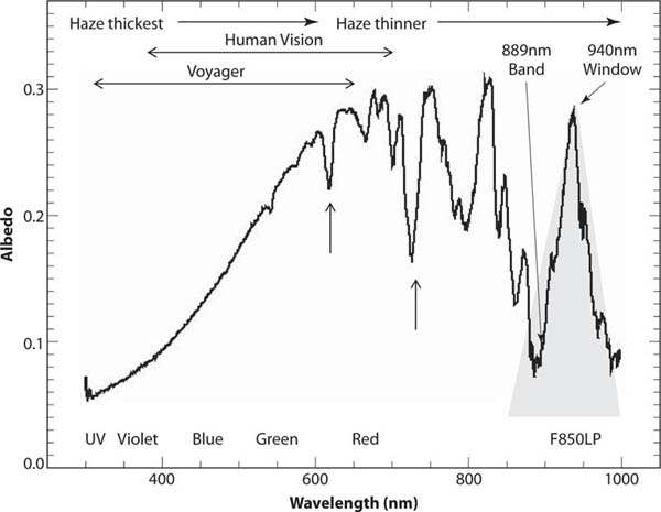
Figure 2.06. A schematic representation of Titan’s reflection spectrum. The albedo is low in the UV and blue due to absorption by the dark haze; the haze is brighter at green, red, and near-infrared wavelengths. In the red and near-IR, progressively wider and deeper methane bands appear. The two arrows show the bands used by Kuiper to discover the atmosphere. The HST image and map in figures 2.01 and 2.02, and all the Cassini surface images in subsequent chapters, are taken through the 940-nm window.

Now, with different detectors, such as those employed in specialized infrared cameras on large telescopes, or on Cassini’s VIMS (visual and infrared mapping spectrometer instrument; see chapter 3), one can exploit the other windows at longer wavelengths where the haze opacity is less. These windows are at 1.07, 1.28, 1.6, 2, 3, and 5 microns. The very small advantage over the 0.94 micron window offered by the one at 1.07 is not worth the added inconvenience of being unable to use a CCD. The 1.28-micron and 1.6-micron windows are rather better, and 2 microns turns out to be the best. The haze is even thinner at 3 and 5 microns than at 2, but there is less and less solar infrared at these longer wavelengths, so exposure times have to be longer. The 2-micron window turns out to be the best compromise. The first map at 2 microns was made by Roland Meier, working with Toby Owen and others in Hawaii using a near-infrared camera, NICMOS, on HST. The map showed impressive contrast, although it was soon surpassed in detail by the much larger telescopes being used for adaptive optics measurements.

 

RALPH’S LOG, FALL 2001

Any book on Titan written before Cassini arrived was, of course, going to be out-of-date post-Cassini. That was never really a concern when we wrote Lifting Titan’s Veil. It was intended largely as a primer on Titan, a report from the coalface of science, and a historical record documenting what our thoughts on Titan were then and why we had them. But some things got out-of-date quicker than expected. One of them was the oft-quoted assertion that the haze hid Titan’s surface entirely from the Voyager cameras.

In the late 1990s, several Titan workers began to wonder if this conclusion was not perhaps too hasty. As they worked with Hubble Space Telescope data and models of Titan’s atmosphere, they began to realize that perhaps a small surface signal might be detectable in visible-light images of Titan. Eliot Young of Southwest Research Institute in Boulder, Colorado, and I were among a number of people suggesting that, should they ever find some spare time (ha!), it might be interesting to revisit the Voyager data.

It actually happened in 2001 in a graduate remote sensing class at the University of Arizona. Alfred McEwen, who is on the Cassini imaging team with responsibility for Titan surface observations, was teaching the class and giving students a small research project. One of the students, Jim Richardson, was assigned the project of trying to find Titan’s surface in Voyager data. Alfred referred Jim to me for help, since I had worked on mapping Titan with HST and was familiar with Titan. Our approach was essentially the same as had been used to make the maps of Titan with HST.

The question was, Had any light got through from the surface in the 600–640-nm wavelength band, the orange light to which the Voyager cameras were just sensitive? In a review paper I wrote with Jonathan Lunine in 1997, we noted that Chris McKay’s radiative transfer code used to study Titan’s atmospheric structure did indicate that Titan’s observed albedo would be sensitive (albeit weakly) to the surface reflectivity at 640 nm, a point that had apparently gone unnoticed. Furthermore, Mark Lemmon’s similar (but independently written) model also indicated such a sensitivity. Additional support came from the suggestion that a partial map made by Peter Smith and colleagues at 673 nm using Hubble Space Telescope images taken in 1994 showed the same broad pattern as that made at 940 nm, which showed much higher contrast. The 673 nm map was only a partial one, as only seven of the fourteen looks at Titan in that observation sequence included 673 nm images; the others were taken up with shorter-wavelength images to study the haze. Had there been more HST time, we might have made a complete 673 nm map, which may have led others to observe more closely at this wavelength too.

It looked like there was a chance. Jim waded through the Voyager image catalogs. The Voyagers took some two hundred images of Titan, although, of course, most appear similar and only a handful of different views are generally shown in papers and books. It turned out that the best images for our purposes were taken with the wide-angle camera, rather than the sharper narrow-angle camera, because the signal-to-noise ratio was better.

Jim used mathematical functions describing the variation of brightness from the center to the limb to boost the contrast of the images. Then, the contribution of a “synthetic atmosphere” of Titan had to be subtracted from the orange images that might have a surface signal buried in them. For our HST mapping, our synthetic average Titan was made just by averaging images from different longitudes. The Voyager images weren’t suitable for this approach, however, so Jim used clear-filter and green-filter images as a background.

The subtraction left a noisy residual picture, with a noticeable north–south asymmetry. Nonetheless, a compelling pair of dark patches looked like they might be real. They were larger than the characteristic mottling of noise. Furthermore, the same patches appeared in three separate Voyager images, in the same places. They also seemed to coincide with some dark regions on the HST 673 nm and 940 nm maps.

In principle, this analysis could have been done when the Voyagers flew by, but one can understand why it was not. Computers then were not what they are now—and say you had found something; could you have believed it, and would anyone else have? Only subsequent weeks and years of Earth-based data showing that identifiable features rotate with Titan make a convincing case that they are indeed surface features.

In any event, the surface data extracted from the Voyager images added little to what was already known but was nevertheless an interesting exercise. Jim Richardson was what is referred to in Britain as a “mature” student. Ironically, given the imaging aspect of this project, he has a guide dog. In a previous career, as a nuclear reactor technician, he lost much of his sight in an industrial accident. His work is an inspiring example to the rest of us.

 

TITAN’S ATMOSPHERE: THE BASICS

Before Cassini, most of our information about Titan’s atmosphere came from Voyager 1. From observations made with Earth-based telescopes, it was known prior to that flyby that Titan has an atmosphere, that it contains methane, and that it is dark in the UV. But it took a close encounter with a spacecraft to learn what a substantial atmosphere it is, what its major constituent is, and how it works.

Voyager’s ultraviolet spectrometer found fluorescence characteristic of molecular nitrogen high in the atmosphere. Then, by measuring the refraction of Voyager’s radio signal to Earth caused by Titan’s atmosphere, it was possible to show that, at Titan’s surface, the atmosphere was about four times denser than the air at sea level on Earth. Additional information came from an infrared spectrometer on Voyager. Taken together, these data showed that the bulk of the atmosphere consists of nitrogen, as is the case for Earth. Titan’s atmosphere was found to be more than 90 percent molecular nitrogen, much of the rest being methane. The surface temperature was measured as around 94 K (−179°C) and the surface pressure as about 1.5 bars. In terms of its vertical temperature structure, Titan looked remarkably like Earth. It was, to be sure, a very cold and vertically stretched version of the Earth, but all the basic features were there. Titan’s atmosphere is far more extended because of the much lower gravity, which is only one-seventh as strong as Earth’s.

From the surface upward, the temperature falls to a minimum value of about 70 K at the tropopause, some 40 km up. (On Earth, temperatures drop similarly with height, but to around −60°C or 213 K at a height of only 10 km above the surface.) This lower layer below the tropopause, the troposphere, holds most of the gas and contributes most of the greenhouse warming in the atmosphere. It is also where weather occurs—vertical motions and the formation of clouds. On Earth, most of the greenhouse effect is due to water vapor, and it is water vapor that condenses to form clouds of water droplets or ice, sometimes to fall down to the ground as rain, hail, or snow. On much colder Titan, the role that water takes on Earth is filled by methane.

Above the tropopause, the temperature increases. This makes the atmosphere stably stratified (hence the name, stratosphere) and little vertical motion occurs. The temperature rise is caused by the absorption of solar radiation. On Earth this is due primarily to ozone, which is formed by the action of solar ultraviolet rays on oxygen. On Titan, the same role is played by the haze. In fact, of the solar radiation falling on the top of Titan’s atmosphere, only about one-third makes it down as far as the tropopause, and only some of that (about 10 percent of the total, or about one-thousandth the amount on Earth) gets down to the surface. So Titan was expected to be a very stagnant sort of place. Because its atmosphere is so thick, not only in density but also in height, it warms up or cools down only very slowly as the seasons change, and temperatures stay nearly constant over time.

Titan’s equator is tilted relative to the path it takes around the Sun, along with Saturn, once every 29.5 Earth years. Titan is tilted only slightly more than Earth is, so it has seasons just like Earth’s, only much longer. One of the most obvious manifestations of the seasons on Titan is a reversing wind pattern that pushes the haze around from one hemisphere to the other. As on Earth, solar heating is, on average, strongest at low latitudes but, during the peak of summer, instantaneously strongest at high latitudes. This heating causes warm air to rise, both on a small scale (producing the “thermals” used by glider pilots and soaring birds) and on a large scale, resulting in a generally cloudy band around the equator. The rising air has to be balanced by sinking elsewhere, and on the rapidly rotating Earth, this is at about 30° latitude in both hemispheres. This symmetric circulation pattern is called the Hadley cell. The descending air is dry, which is why we find our deserts at around 30° latitude.

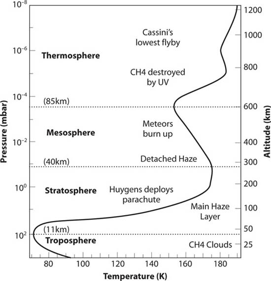
Figure 2.07. Titan’s atmospheric structure, which resembles that of the Earth (albeit vertically stretched and much colder).

Slowly rotating Titan’s sluggish atmosphere behaves a little differently. In the stratosphere at least, where much of the Sun’s radiation is absorbed, the flow rises over the summer hemisphere and descends over the winter one, In effect, there is a pole-to-pole Hadley cell. This situation seems to persist for almost half a Titan year. Then, at the equinox, as the subsolar latitude crosses the equator, the circulation must cease and reverse direction. In so doing, models suggest, Titan may have a brief inter-lude, lasting an Earth year or two, when there is a vaguely symmetric Earth-like circulation, with rising at the equator and sinking in both hemispheres, before the reversed pole-to-pole motion takes over.

Figure 2.08. The meridional Hadley circulation during Titan summer. The warm air rises, perhaps causing clouds to form, and drags haze into the winter hemisphere. Unusual effects occur over the winter pole where low-temperature downward circulation brings organic compounds and haze down to lower altitudes.

The summer-to-winter motion must drag some haze with it, and indeed this is just what has been observed. Haze makes the atmosphere bright in the near-infrared, especially in the methane bands (where the haze is bright and above the absorbing lower atmosphere), and dark at blue-green wavelengths (where the gas would be bright but the haze is dark). So, a more hazy part of the atmosphere looks redder than a less hazy part—dark in blue light, bright in the near-IR.

When Voyager flew past Titan in 1980, the southern hemisphere was brighter to its cameras, which were primarily sensitive to short-wavelength light in the blue and green. When HST observed Titan in the 1990s, the situation was exactly reversed. The north was brighter. The appearance in the near-infrared (which Voyager could not see) was very different. First, instead of the limb (that is, the periphery of the visible disk) being darker, the limb was bright. It is easy to work out why. The haze is thinly distributed in a shell around Titan, so, viewing the edge of the disk, you look through a longer slanting path of haze than when you look straight down at the center of the disk. What you see is light scattered by the haze. More haze at the edge means more light. Hence, the limb is bright in the methane bands, giving Titan a ringlike appearance. But it is not a symmetric ring. In the HST observations, more haze was in the south, and so the southern limb was brighter and thicker than the northern one. Titan appeared to have a smile.

Figure 2.09. An image of Titan from Voyager 2 (somewhat stretched in contrast compared with figure 1.03). The enhanced contrast brings out the polar collar, as well as the difference in brightness between the hemispheres. The detached haze is also weakly visible at the left limb. (NASA)

As the models predicted though, the pole-to-pole Hadley circulation would drag haze back from south to north, and in the years around the turn of the millennium, the situation would reverse. In the twenty-first century, Titan quickly began to resemble once more how it had appeared to Voyager in the early 1980s, with the southern hemisphere bright in the blue. In the near-infrared, the smile became a frown.

The slow Hadley circulation of north–south winds is responsible for Titan’s seasonal changes, but much faster zonal (east–west) winds are important too. These have the effect of shearing out clouds as they puff their way upward, and as we will see in chapter 6, they also manifest themselves in the transport of sand across the surface of Titan. They were important in the design of the Huygens probe’s mission because the probe would drift several hundreds of kilometers eastward as it descended. These strong zonal winds occur to some extent on Earth (the jet stream that affects air travel across the Atlantic being an example), but they are most apparent in optically thick atmospheres, such as those of the giant planets or totally overcast Venus.

Figure 2.10. A collection of visible and near-visible images from the Hubble Space Telescope for the years 1992–2002. From left to right, they are near-UV (336 nm), blue, green, red methane band, red continuum, near-IR methane band (889 nm), and near-IR continuum (953 nm). The most prominent seasonal changes are in the blue sequence, where the brighter northern hemisphere progressively darkens relative to the southern one, and in the near-IR methane band images, where the “smile” becomes a frown as high-altitude haze migrates to the northern winter hemisphere. (R. Lorenz/STScI)

The first indications of the zonal winds were the deduction from Voyager infrared data that the equator-to-pole temperature gradient in the stratosphere required strong zonal winds for the pressure gradient to balance out. Although indirect, this model of Titan’s zonal winds, developed by Mike Flasar of the Goddard Space Flight Center in Maryland, proved to be pretty close to the mark, suggesting winds of the order of 100 m/s in the stratosphere. Some additional support to the model came in 1989, when Titan occulted the star 28 Sagitarii (see later in this chapter).

So Titan, with its atmosphere, is in some ways a strange analogue of our home planet, the role of water being taken by methane. Titan is sometimes compared with the early Earth, before life and the appearance of oxygen. However, much warmer Earth was probably never as hydrogen-rich as is Titan, so this comparison shouldn’t be taken too far. Nevertheless, the differences between the prebiotic Earth and the present Earth are certainly similar in nature to the differences between Titan and the present Earth, so there is doubtless much to be learned from processes on Titan that is relevant to understanding the evolution of Earth.

TITAN’S ATMOSPHERIC CHEMICAL FACTORY

Despite the similarities, Titan’s atmosphere is very different from Earth’s with respect to chemistry. Even before Cassini, some twenty different organic compounds made of carbon, nitrogen, and hydrogen had been identified in Titan’s atmosphere. These are nearly all made by the action of ultraviolet light on methane, aided and abetted, particularly for the nitrogen-bearing compounds, by cosmic rays and electrons trapped by Saturn’s magnetic field. The simplest and most abundant ones include ethane, propane, and acetylene, all of which are present in natural gas on Earth. Also prominent is the poisonous gas hydrogen cyanide, at a level of about one part per million, not quite a toxic concentration for us. Many other more complicated molecules were detected from their infrared spectral signatures.

In contrast, oxygen-bearing molecules are conspicuous by their absence. The most abundant is the most volatile—namely, carbon monoxide—a gas also found in comets and probably around since Titan’s formation. But less volatile oxygen-bearing species such as carbon dioxide and water are present only as traces—a few parts per billion. Even though these are very common in the warm inner solar system, at Titan they behave physically more like rock—hardly the stuff of an atmosphere. In fact, the traces that we do see in Titan’s stratosphere probably did not come from Titan’s surface, but from above, delivered as icy meteoroids that “burned up” as they lanced into the upper atmosphere. Some of the water thereby introduced is converted, again by solar ultraviolet-driven chemistry, into carbon dioxide. That we are able to detect the presence of these compounds at all is an impressive achievement. In abundance terms, they are present at the sort of level that man-made chlorofluorocarbons are present in Earth’s atmosphere.

TABLE 2.01
Composition of Titan’s Atmosphere

Tiny though the traces are, the amount of CO₂ in Titan’s atmosphere appeared to demand rather more water to be delivered to Titan’s atmosphere than was expected from models of how many meteoroids there should be. As we will see, this anomaly presaged later findings about the remarkable amount and mobility of water in the Saturnian system.

Figure 2.11. A close-up of Titan’s northern hemisphere from Voyager 1. The polar hood appears to stand up above the main haze deck, and extends southward as a detached haze layer. (NASA)

Titan’s atmospheric chemistry is not uniform and varies with both latitude and altitude. Since many molecules are produced by photochemistry high up, they are most abundant at high altitudes, and at latitudes where downward winds bring air from higher, more enriched levels. This happens most graphically during polar winter and is marked not only by a tenfold enhancement of the concentration of some gases but also by a dark region of concentrated haze. This haze seems distinct from that over the rest of Titan, having different spectral properties, perhaps because some compounds have condensed onto the haze particles during the polar winter. This phenomenon, called the dark polar hood, has some intriguing parallels on Earth. Here, the long winter night causes clouds of ice crystals to form, known as polar stratospheric clouds, and chemistry on the catalytic surfaces of the ice crystals results in local depletion of ozone. This ozone “hole” is isolated from the rest of the atmosphere by zonal winds, the so-called circumpolar vortex, which blocks flow to or from lower latitudes. Of course, the chemistry is very different on Titan (and indeed the dominant physical processes are too), but a detailed investigation of the polar hood is likely to be instructive for understanding the Earth too.

The polar hood was observed by Voyager 1, at the northern spring equinox, as a dark circle poleward of about 65° north. At the equinox, both polar regions were illuminated and visible, but there was no such feature in the south. From Earth, little could be seen with HST when Titan was observed around the southern spring equinox in 1995. The HST images had a much lower resolution than the Voyager ones, and the polar region was right at the edge of the disk. However, as time went on, the south pole became more and more visible, and sure enough, a polar hood was apparent by the end of the 1990s. HST was equipped with a new camera in 2002, one able to produce better images in the ultraviolet than before, and it is at ultraviolet wavelengths that the hood shows strongest contrast. The hood was very prominent in the UV in 2002, but by 2003 it was beginning to fade. Of course, if Titan’s appearance varies in the same way through each cycle of seasons, then the south polar hood would have to disappear by 2009 in order for Titan to look like it did in 1980. By the time Cassini arrived in 2004, it had in fact disappeared altogether.

LOOKING FOR A NATURAL GAS SUPPLY

We’ve discussed how sunlight breaks down methane in Titan’s atmosphere and turns it into ethane, acetylene, and other materials, notably the haze. But scientists interpreting the Voyager data realized that the entire inventory of methane in Titan’s atmosphere would be destroyed this way in only about ten million years, or a fraction of the age of the solar system. So why was the methane still there?

Attention was drawn by the near-coincidence of Titan’s surface temperature with the triple point of methane. At the triple point, materials can coexist in their solid, liquid, and vapor phases, and it so happens that Earth’s average temperature is not far off the triple point of water, which is close to the freezing point of 273 K. The basic physics is straightforward, although there are some subtle and interesting feedbacks at work that have maintained Earth’s temperature close to its present level for all of solar system history, even though the Sun was probably 30 percent fainter at the beginning. It takes energy (or “latent heat”) to convert ice to water and water to steam. That is why ice cubes are good for cooling drinks, and why it takes a kettle a long time to boil dry. Much of the heat reaching Earth from the Sun goes into these phase changes, especially evaporating water, which drives the hydrological cycle. In cooler areas, the water condenses and falls as rain or snow, ultimately to be evaporated again and so on.

So, if Titan’s temperature were close to the methane triple point, perhaps phase changes were buffering the temperature. By implication, phases other than the vapor one would be present. In other words, there might be liquid methane at the surface. The Voyager temperature and pressure data couldn’t say for sure, but if there were seas of liquid methane on Titan, their slow evaporation could perhaps keep resupplying the atmosphere against the steady destruction by sunlight. Over 4.5 billion years, this process might use up around a kilometer depth of a global methane ocean. Such an amount—compare it with the 4 km average depth of the Earth’s water oceans—was not implausible, but a 1-km-deep ocean would probably submerge most of Titan’s topography. At most, there would be a few islands poking up before waves and tides wore them down.

It became clear in the 1990s, as near-infrared maps showed Titan to have bright and dark regions on its surface, and radar showed the surface was generally too radar-reflective to be covered in liquid hydrocarbons, that this global ocean model, appealing as it was, could no longer hold. Another idea put forward to solve the methane supply problem was that it is being continuously released from the interior, by volcanoes or geysers.

However, that didn’t make Titan dry. The models of Titan’s photochemistry, though they had all kinds of questionable assumptions in the detail, were, broadly speaking, pretty robust and predicted that most of the methane should be converted into ethane, which is also liquid at Titan’s surface. Though ethane is produced only slowly by the atmospheric photochemistry, over the age of the solar system, several hundred meters’ worth would be expected, along with a few hundred meters of solid stuff. The problem was not just finding some way of resupplying the atmospheric methane but also of disposing the ethane thereby produced.

Another inconvenient aspect of the no-ocean-volcanoes-instead model was that, unless the methane delivery rate was very finely tuned to match exactly the photochemical destruction rate, which varied through time as the Sun’s brightness and color evolved, methane would accumulate anyway to the point where it would condense into lakes or seas, or it would be temporarily exhausted. The ideas of the Voyager era therefore faltered in the face of Titan’s complex reality.

In space or time, somehow the picture is more complicated. Perhaps there is lots of liquid methane and ethane on Titan, but hidden in caverns and porespace beneath the visible surface, like the groundwater aquifers on Earth. Or perhaps, instead of drizzling down uniformly everywhere, the ethane has been dumped at Titan’s high latitudes, which could not be seen from Earth, and maybe most of the methane is there too. Or maybe there hasn’t been methane in Titan’s atmosphere for all time—that would make for some interesting climate change through Titan’s history, since the methane greenhouse effect is responsible for keeping Titan some 12 K warmer than it would otherwise be—in which case the ethane disposal problem is easier. Even with Cassini, this puzzle has not yet been solved.

RADAR AND THE CASE FOR SEAS

A compelling piece of evidence in favor of seas on Titan came in 2002, when Titan moved into the sights of the giant Arecibo radio dish, operated by a group led by Don Campbell of Cornell University. Because this giant 300-m radio telescope is built into the ground, it can only observe over a narrow range of sky close to the overhead direction and so relies on planetary motion and the Earth’s rotation to capture its targets. When Titan drew into view at Arecibo, the telescope had recently been upgraded with more powerful radar transmitters and sensitive receivers that would be able to do far better than Goldstone/Very Large Array (VLA) radar experiments carried out in the early 1990s.

These improvements meant that the signal-to-noise ratio was far higher. A measurement of the reflectivity of the disk taken as a whole would be more accurate and believable than the albedo determined before. And there was even enough signal to allow the echo to be chopped up in frequency and time.

The reason for separating different frequencies in the received signal is as follows. Titan spins with its rotation axis approximately orthogonal to the line joining Titan and Earth, so the morning edge of Titan is coming toward us while the evening side recedes. Thus, echoes from the morning side of Titan have a blue shift because the Doppler effect moves signal to a slightly higher frequency, whereas the opposite occurs on the evening limb. This allows us to measure how much of the echo is coming from the morning and evening parts of the disk, and how much from the center, which is moving neither toward nor away from us. (Of course, due to Earth’s rotation, its motion around the Sun, Saturn’s motion around the Sun, and Titan’s motion around Saturn, Titan’s center is approaching or receding from us, but this is all taken into account separately.)

The radio telescope sent out a powerful microwave beam, at a single frequency. The beam’s power was something like a megawatt. The Doppler spreading of the echo due to Titan’s rotation caused most of the echo power to come back in a broad, hump-shaped spectrum with a bandwidth of about 375 Hz.

But strikingly, the Titan echoes had a unique feature. There was sometimes a strong spike in the Doppler spectrum, as if a very strong echo were coming back from just a narrow region in frequency space—in other words, from a small region on Titan. The only way this could realistically happen is if there were regions on Titan that are flat on the scale of the radar wavelength, so that there was a mirrorlike reflection.

So-called specular reflections like this are routinely seen by weather satellites on Earth’s oceans, though only where the sea surface is calm. Although the intrinsic reflectivity of the ocean isn’t in fact very high (which is why you can see a shallow seabed), the geometry of a specular reflection makes it appear very bright. And so it was with the Arecibo spike echoes. Although they were striking, the actual reflectivity calculated was quite low. These were dark mirrors.

A lake of liquid ethane seemed like an obvious, and appealing, explanation. And since photochemical models suggested that we should find lakes and seas of liquid hydrocarbons, the facts seemed to fit. But as always, there were other possibilities. A flat, organic-rich plain acting as a dark mirror could be all kinds of things, not just a lake of ethane with fluid properties much like gasoline at terrestrial temperatures. It might be a flat lakebed like the playas in the desert Southwest, but covered in a thick organic tar. Or it could be heterogeneous on scales smaller than the radar could see—small patches of bright, smooth reflection (flat ice, perhaps) dotted over a rough surface.

 

RALPH’S LOG, 2003

Because the radar observation of Titan was made possible by changing planetary geometry, with Titan slowly drifting into the sights of the Arecibo dish, it reminded me of a scene in the original Star Wars film (episode 4—“A New Hope”). The film’s tense ending is paced by the inexorable motions of the Death Star and the jungle moon (Yavin 4), both in orbit around the giant planet Yavin. If the rebel heroes don’t disable the Death Star in time, the moon, and the secret rebel base on it, will drift into the sights of the Death Star’s super-laser (looking like a huge dish), and all will be lost.

While writing a commentary article for Science magazine to accompany the Campbell et al. paper, I cheekily threw in a reference to Yavin 4. This generated me some kudos among some of my planetary science colleagues, who, it must be admitted, are sci-fi fans. I am not aware of any other scientific publications mentioning this fictitious world. Some years later, findings on Titan would prompt me to write about another sci-fi word, “Arrakis,” better known as “Dune.”

 

ANTICIPATING THE LANDSCAPE

Speculations about Titan’s landscape had ranged from the exotic global ocean of hydrocarbons to a rather bleak and dull cratered iceball, like Callisto with an atmosphere. However, the variegated pattern of brightness at least showed that something was happening on Titan to make some areas light and some dark; but without any data to inform the speculations, they remained just that. It was possible to make some guesses—if so-and-so happened on Titan, then Titan’s environment would be like this. One could, for example, anticipate how many impact craters Titan should have, by analogy with the crater populations seen elsewhere in the solar system. Titan would have very few small craters. Normally, small craters are the most abundant because the small comets and asteroids that make them are more common than big ones. But on Titan, small comets would break up in the atmosphere, as happened in the case of the Tunguska explosion in Siberia in 1908. Or, given the thick atmosphere and modest solubility of methane gas in water, one could predict that any volcanoes were more likely to be dome- or shield-shaped, rather than graceful cones like Mount Fuji: there wouldn’t be enough gas to spray out “ash” fast enough to build a cone.

But it is not so much the character of individual processes like those just mentioned that would define what Titan’s surface was like, but rather the balance between them. In the absence of any other information, one could at least estimate the amount of energy expended in different processes, considering the atmosphere and the planetary interior as engines that worked the landscape, driven by heat. Although it was difficult to relate a given type of feature to a given amount of work, at least the relative strengths of the processes could give some estimate of the land-forms likely to dominate.

Consider the case of Earth, for example. About 80 mW m⁻² of heat leaks out of Earth’s interior and is involved with the tectonic forces that push up mountains like the Himalayas and Alps, as well as more directly in the formation of volcanoes. A much higher amount of heat, about 20 W m⁻², flows across Earth’s surface and drives ocean currents, winds, and waves. Maybe 1 W m⁻² is expressed as the tides in the ocean. And if the explosive energy in occasional impacts—one meteor crater of 1-km diameter every fifty thousand years, one dinosaur-killer every fifty million years, and so on—is added up, it amounts to only microwatts per square meter. Although each of these processes has a certain amount of energy associated with it, characterized by a numerical value, the efficiency of each in modifying the landscape is rather different. Impact cratering directly sculpts the surface, whereas the much larger atmospheric flows must find tools like gravel in rivers to make a mark on the landscape. But the progression of decreasing power, from atmospheric through tidal and volcanotectonic to cratering processes, is what defines our landscape. After all, impact craters occupy only a small fraction of Earth’s surface, but river valleys and sand dunes occupy much.

The same calculation could be done for Titan. We know the amount of sunlight reaching the surface to drive the weather, and we know roughly the amount of rock and thus the amount of radioactive heat produced in the interior, which defines the volcanic/tectonic output. From these considerations, one finds the same progression: atmospheric—tidal—volcanotectonic—cratering, albeit with much smaller numerical values. Maybe the numerical values wouldn’t matter so much, since Titan is made of more volatile, perhaps more easily worked, materials like ice and organics instead of rock. It was hard to say. Of most significance was the fact that the dynamic range of energies involved, the factor by which the atmosphere was stronger than the volcanotectonic work rate, and so on, was much smaller than that for Earth. In other words, Titan’s competing processes were more closely balanced than on Earth, suggesting that we would see a varied landscape.

A CLOUD OR TWO IN THE SKY

The improved telescopic observations of the 1990s shed light on one particular aspect of Titan’s atmosphere. The detection of clouds indicated the existence of a methane “hydrological” cycle. It’s worth emphasizing here an important difference between ethane and methane. Although both are gases at terrestrial temperatures, the boiling point of ethane is much higher than that of methane and it is essentially involatile at Titan’s surface temperatures. Whereas methane can evaporate and form enough vapor to subsequently condense into clouds or rain, ethane just sits there. In principle, there might be ethane lakes—very old ones—but never ethane rivers. Any rivers would have to be created by methane rainfall.

The first firm observations of clouds, made in 1995 and 1998 by Caitlin Griffith and Toby Owen, relied on ground-based spectroscopy, which showed that Titan’s brightness occasionally varied when measured at wavelengths at the edges of the methane bands. This was distinct from the regular, predictable variation in brightness observed in the windows between the bands due to the bright and dark regions on the surface coming into view as Titan rotated. These occasional variations could be dramatic over just a few hours. Further, by the way they differed between wavelengths, their location could be narrowed down to an altitude range between 10 and 30 km, just where methane would be expected to condense.

The fact that there were variations on timescales as short as a few hours suggested that these were convecting clouds, like the cauliflower cumulus clouds that puff up on a summer day on Earth. After the clouds blossom upward, rain forms in them and they dissipate. In fact, it turned out that HST had observed a large cloud at around 40° north in 1995, which was also broadly consistent with clouds being driven by direct solar heating. So, the changing clouds on Titan suggested an active weather cycle. However, it was known from Voyager that the lower atmosphere was not saturated with methane, so raindrops, which would fall slowly in Titan’s low gravity, might evaporate before they hit the ground. Clouds didn’t necessarily imply rain on the surface.

Figure 2.12. Titan’s methane cycle. After its introduction into the surface—atmosphere system, perhaps through volcanic vents, methane participates in a slow hydrological cycle involving clouds, rain, and rivers. Some methane leaks up into the stratosphere, where it is converted into ethane liquid, which collects in lakes near the poles, and heavier solid organics, which drizzle down to the surface.

Titan’s clouds turn out to be rather elusive and transitory. Part of the reason why they were hard to spot in the first place and why there have been few detections is that they aren’t always there. That sounds trivial, but without continuous monitoring it is impossible to know and it is difficult to justify looking for something with an expensive and oversubscribed telescope unless you already have good evidence that you’ll find it. So there was a chicken-and-egg problem over studying clouds if reliance was placed on the usual systems for allotting telescope time.

A keen observer might be able to get a run of a few nights on a telescope equipped to detect clouds on Titan. A generous allocation might be ten nights a year, but some of those could be hampered by bad weather on Earth or equipment problems. Let’s say that Titan has visible clouds about half the time. If that were the case, there would still be a good chance of seeing clouds on at least a couple of nights. But clouds on Titan, it seems, are scarcer than that. Earth’s cloud cover is about 30 percent, but some theoretical models of Titan’s clouds and how often the weak sunlight can drive the upward convective air motions suggested a cloud cover of only a few percent. Multiply that by the number of nights of observing, and the odds of discovery are not so good.

The spectroscopic discovery of clouds at least showed they existed sometimes. But the fact that not all observers had seen them was a challenge and left us with no real idea of how big or how often methane storms were. It took some creative thinking to come up with a solution.

Astronomers, especially those studying distant galaxies or other faint objects, are used to long nights at the telescope, often staring at a tiny piece of sky to gather up every scrap of light. Or they are engaged in surveys, gathering statistics on large numbers of stars or asteroids. And so, telescope time is often allocated in blocks of whole or half nights. But with large telescopes, such as the Kecks, getting a good set of Titan images need take only fifteen minutes or so. But no formal way to get time in such short blocks exists.

In 2002, Antonin Bouchez at Caltech (and subsequently at the Keck Observatory itself), together with Mike Brown, came up with two clever approaches. First, Bouchez set up a command script at the Keck with all the right filter and adaptive optics settings, such that any regular observer could take a set of Titan images relatively easily if they happened to have some minutes to spare, perhaps before their intended target had risen high enough in the sky, or after they had got all the data they needed. Second, they found a way of getting at least a hint that there might be clouds worth seeing.

The early-warning system involved a fourteen-inch “amateur” telescope on the roof at Caltech and, more important, talented and hardworking graduate students Sarah Horst and Emily Schaller. Although viewing conditions in the brightly lit and smoggy Los Angeles megopolis are hardly ideal, it was possible to take images of the Saturnian system with a CCD camera through two filters—one transmitting radiation inside a methane band and one in the nearby continuum. The murky skies make it a challenge to decide whether Titan is anomalously bright or not in an individual image, but assuming terrestrial murk affects both wavelengths the same, the ratio between Titan’s brightness in the continuum and the band gives a much more robust measurement.

Even this was pushing the limit of what is reproducible. But after some months of observing, they had enough experience and statistics to be able to pull out Titan’s underlying lightcurve and to see if Titan was anomalously bright. Armed with that information, a call to the Keck control room netted them a good number of cloud detections. Perhaps they were assisted by the fact that it was midsummer over Titan’s exposed south pole in 2002–3, and clouds were bubbling up all the time.

This work stands as a remarkable example of what can be achieved with amateur equipment and some hard work. With the proof-of-concept (and proof in the results), this important program continues, now using a larger remotely controlled telescope in Arizona.

So ultimately, after the first, essentially unverifiable, reports of clouds on Titan in the 1990s, the large AO systems of the twenty-first century are routinely and unambiguously detecting clouds on Titan.

EXPLOITING TITAN’S OCCULTATIONS

Occasionally, nature offers us an opportunity to secure high-resolution information about a moon or planet, even with a small telescope. For example, moons, planets, and asteroids are sometimes occulted by other solar system objects, especially the Earth’s Moon. Jim Elliott of the Massachusetts Institute of Technology observed lunar occultations of Titan in 1974 and used his data to calculate a value for Titan’s diameter.

Elliott’s value of 5,800 km turned out to be an overestimate. Measuring Titan’s size is complicated by the fact that Titan has an atmosphere. Not only is its edge fuzzy, its perceived diameter is not the same at all wavelengths. Since blue light is more effectively absorbed by the haze, the apparent diameter is larger in blue light than in red or near-infrared. The same wavelength effect was seen in images of Titan’s shadow cast onto Saturn in 1995. At that time, Saturn’s rings were presented edge-on, and when Titan was in front of Saturn, its shadow was projected onto the planet’s disk. After taking into account that Titan’s shadow was being cast onto the curved surface of Saturn’s cloud deck, scientists were able to measure Titan’s diameter at a range of wavelengths and to see that the distribution of haze with altitude wasn’t the same all around the disk.

On occasion, Titan has itself been the occulting body, blocking out the light from a star for a short while. Precise timing of how long the star winks out during such an occultation can define the diameter of an occulting body quite accurately, even if the body itself cannot actually be resolved with the telescope making the observation. Furthermore, if the occulting object has an atmosphere, as in the case of Titan, the way in which the starlight gradually declines at the start of the occultation, then rises again at the end, can be analyzed for information about the structure of the atmosphere.

Figure 2.13. An HST image of Titan (at left) and Saturn, during the ring-plane crossing season (southern spring equinox) in late 1995. The rings are seen edge-on, and several other moons are visible on the right. The unique aspect of this picture is the shadow of Titan cast onto Saturn. Careful study of the shape of the shadow revealed characteristics of the haze distribution that would otherwise be impossible to detect. (E. Karkoschka/STScI/University of Arizona)

In effect, the atmosphere behaves as a lens. As the beam of starlight travels through the atmosphere, its path is bent. Its intensity varies with time as it scans through different levels of the atmosphere allowing the density (or more strictly, the refractivity) to be measured. From this the temperature structure can be inferred. The technique only works over a specific range of altitudes—those where the air density is high enough to produce measurable bending, but not where the gas or haze absorbs the light to undetectable levels. Spikes in the lightcurve can also indicate local inhomogeneities in the atmosphere, such as gravity waves. On Titan, the altitude range probed by occultations is between about 250 and 450 km.

A major occultation event occurred on July 3, 1989, when Titan crossed in front of the star 28 Sagittarii. At magnitude 5.5, 28 Sag was bright enough to be seen by the naked eye under good observing conditions. Such an occultation is sufficiently rare and of such potential importance, considerable effort was put into the preparations to observe it. Larry H. Wasserman of the Lowell Observatory predicted that the occultation would be visible from Europe, but considerable uncertainties were inherent in the calculations. No one could be confident about what would actually be seen from any particular place. For once, astronomers found their luck was in. The prediction of when and where the occultation would be visible was pretty accurate and skies were clear. The event was recorded from as far north as Sweden to the Pic du Midi Observatory in the Pyrenees Mountains of southern France.

The intensity of starlight declined over about twenty seconds as anticipated, complete with “spikes,” but then there was a total surprise. The occultation was expected to last some five minutes. About halfway through, there was a bright flash as if the star were shining through Titan. In fact, as the star got close to being directly behind the center of Titan, its light was being bent around the entire limb of Titan. The flash lasted around five seconds at Paris and a shorter time elsewhere. The shape and timing of the central flash provided a bonus of additional information about the atmosphere.

If Titan’s atmosphere were perfectly uniform, a ring of images would be formed. As shown by a careful analysis of the data from this event, Titan’s atmosphere seemed to act as if deformed by rapid rotation into an oblate spheroid, allowing in principle four simultaneous images of the star. The oblateness of the 250-microbar contour in Titan’s atmosphere revealed by the occultation confirmed that the upper atmosphere must be rotating fairly fast, with zonal winds of perhaps 100 m/s at high altitudes, causing the atmosphere to deform. This was a valuable piece of information, confirming the indirect suggestion from the Voyager temperature measurements that Titan should have strong zonal winds. These meant that the Huygens probe could expect to drift several hundreds of kilometers during its descent.

Although occultations by Titan of a star as bright as 28 Sag would be expected once every fifty thousand years, seeing a central flash would be expected only once every million years! This was indeed a remarkably fortuitous coincidence. But more opportunities for stellar occultation observations followed, even if they were less spectacular.

The occultation of a much dimmer star took place in 1995, and an analysis showed Titan to be slightly off-center optically (compared with 1989). This suggested that the structure of the haze in relation to latitude was changing, just as the HST images were showing.

A rather favorable occultation occurred on December 20, 2001, when a 12.4-magnitude star was occulted by Titan high over the United States. Although this star was too faint for most amateur telescopes, an arsenal of large telescopes was aimed at Titan, in particular the two-hundred-inch Palomar telescope with its new adaptive optics system.

Figure 2.14. A sequence of images from a near-infrared adaptive optics movie acquired by Antonin Bouchez and colleagues at the Palomar two-hundred-inch telescope in late 2001. Titan’s disk is clearly resolved, and the Xanadu bright feature is seen at the center. Titan was observed moving across a pair of stars (although all these images are centered on Titan). In some of the images, the stars are visible as bumps on the edge of the disk. Their precise position and brightness when close to the disk gave a picture of the structure of Titan’s atmosphere. (Antonin Bouchez/Caltech)

The team there, led by graduate student Antonin Bouchez from Caltech, was lucky. The weather and the equipment both cooperated. Titan was seen as a disk, with Xanadu visible. The star was an unremarkable object, looked at in any detail only because Titan happened to pass in front of it (an unlikely claim to stellar fame); but it turned out to be two stars! They were separated by only a little over an arcsecond, so the regular telescopes that had observed it previously had not recognized it as a close pair of distinct stars. Bouchez feared for a while that there might be no occultation at all, that Titan might pass between the two stars.

Luckily, the alignment was almost perfect, and Titan moved across the two stars in turn. The first winked briefly as Titan’s atmosphere passed in front, and its image could then be seen moving along the northern edge of Titan, before reemerging on the other side. The second star hit a little farther south, and its image passed along the southern limb. At some moments, the symmetry of the atmosphere allowed two images of the star to show, on opposite sides. Although neither star was close enough to dead center to cause a central flash, having the primary images of the stars in opposite hemispheres gave a global sampling of the atmosphere.

Less cinematographic, but nonetheless important, was a pair of occultations on November 14, 2003. These were the last chance to observe Titan this way before Cassini arrived, and mission planners were concerned about gravity waves in Titan’s atmosphere. These periodic fluctuations in density might, if large enough and caught at an unlucky moment, cause the Huygens probe to trigger its parachute too early, possibly outside the regime where it would survive. Since gravity waves could be detected by the scintillations in an occultation, confirming that these fluctuations were not too large would give a useful boost to confidence in the mission.

The first of the occultations was of a fairly bright star of magnitude 8.6, within the reach of amateur telescopes. However, it was observable only in the more remote Southern Hemisphere. Observers, led by Bruno Sicardy of the Paris Observatory, set up a “fence” of telescopes in Namibia, South Africa, and Madagascar, with the hope of capturing the all-important central flash. Several telescopes caught it, with some adjacent telescopes making lightcurves at different wavelengths.

Later that night, when Titan could be observed over North America, a less generous 10.4-magnitude star was occulted. However, bad weather thwarted most observers (including the first author of this book, surrounded by clouds on Mt. Bigelow).

TAKING TITAN’S X-RAY

On January 5, 2003, Titan executed a truly bizarre occultation when it drifted in front of one of the most exotic and energetic objects in the sky—the Crab Nebula. This object is a supernova remnant, which was formed in the year a.d. 1054 by the explosion of a star that was witnessed and recorded by Chinese and Arab astronomers. The remains of the star itself are a pulsar at the heart of the nebula. Powered by high-speed electrons emitted by the pulsar, the nebula is one of the strongest radio sources in the sky and also a source of X-rays. The alignment of Titan and the Crab in 2003 was the first since the nebula was formed. The next will not occur until 2267. Fortunately, the once-in-a-millennium event was observed by the Chandra X-ray Observatory, a 20-m-long five-ton spacecraft launched in 1999 from the space shuttle into an orbit 10,000 km above Earth.

Figure 2.15. An image by the Chandra X-ray Observatory of the Crab Nebula, which is a bright, extended X-ray source. On January 5, 2003, Titan crossed in front of the nebula, and processing of the data allowed the one-arcsecond-diameter X-ray shadow cast by the moon (inset) to be reconstructed. (NASA/CXC/Penn State/K. Mori et al.)

Koji Mori of Pennsylvania State University and his colleagues observed the Crab with Chandra for nine hours as Titan swept across. Even though the Crab is a powerful source, there are so few X-ray photons that one can’t just see the shadow of Titan. Mori and his team reprojected the position of each photon onto a reference frame attached to Titan, in effect unsmearing Titan’s motion across the nebula. After that, they had to consider how much the telescope itself smeared out the shadow.

They found that the X-ray shadow was about 0.588 arcseconds across, implying that the altitude above Titan’s surface below which the X-rays were blocked was about 880 km. This is much higher than the altitude of 200 km below which visible light is blocked. The explanation is that X-rays, although better than light at penetrating short distances through solids, are less effective at penetrating long distances through air.

When scientists compared this atmospheric thickness with what would be expected from the models based on Voyager data, it seemed that Titan’s atmosphere was a little thicker. Perhaps it had warmed and puffed up a little because Titan was closer to the Sun.

The planetary science community working on Titan had, of course, never crossed paths with these X-ray astronomers before. It was an ingenious observation, indeed, but no one had a good sense of how much to believe the results. Was the observation or its interpretation suspect, or had the atmosphere really puffed up? Perhaps it wouldn’t be a surprise to learn that it had, since Saturn’s orbit around the Sun is appreciably eccentric and Titan was closer to the Sun than it was when Voyager flew by.

INSIDE TITAN

Although the details of Titan’s surface remained elusive, at least some good theories were put forth about Titan’s overall composition and the structure of its interior. The way we think planets and moons form is by collision of much smaller chunks of matter called planetesimals. These in turn are made of rock and ice, ultimately themselves made of tiny particles that stuck together in the swirling cloud of dust and gas around the Sun when the solar system formed. The proportion of rock, metal, ice, and frozen gases in these planetesimals presumably varied throughout the solar system, with the inner solar system dominated by rock and metal so as to give rise to the dense terrestrial planets. But further than about 4 AU from the Sun, beyond the so-called snow line, water ice becomes abundant, so most of the satellites in the outer solar system are icy. And water ice, if cold enough, can also trap gases such as ammonia and methane.

Each of the giant planets’ retinues of satellites is a solar system in miniature. As the planetesimals (with whatever composition is characteristic of that distance from the Sun) float along in their orbits around the nascent planet, they begin to clump together, sticking like snowballs. But as the clumps become bigger, their gravity draws other planetesimals in at faster speeds, and soon they begin to smash together. As a satellite grows, the collision energy increases, to the point where incoming planetesimals are heated by their impacts such that the ice melts. And so, the growing Titan began as a core of gas-laden ice and rock, but was then surrounded by a layer of rock, where the rocky material in the later planetesimals had fallen through the molten ice. This, in turn, was overlain by a layer of liquid water and capped with a primitive atmosphere. That initial hot atmosphere probably had little in common with the atmosphere we see today, being richer in water vapor and ammonia.

It sounds like a rather fancy story, supported by little more than the observation that many outer solar system satellites are icy. But the pattern seen in the solar system is repeated in microcosm around each giant planet, suggesting the formation process is rather consistent with the picture above.

Gravity measurements by the Galileo spacecraft in the late 1990s began to show the overall structure of Jupiter’s Galilean moons. Superimposed on the issue of bulk composition (Io being all rock, ice, and sulphur; Europa being like an Io with a 100-km veneer of liquid water and ice; and Ganymede and Callisto being more like half rock and half ice) is the question of how much their interiors have sorted themselves out. Even though the bulk ice fraction increases as one moves away from Jupiter, the ice fraction in the exposed surface (roughly indicated by the optical or radar reflectivity) decreases. Europa is so bright presumably because its surface is covered in fresh frost, whereas Callisto is dead and dark.

The question naturally arises as to why Titan has an atmosphere when Ganymede and Callisto do not. A number of factors are at work, and it is not really known which are the most important. First, the composition of the warm Jovian nebula was probably less volatile-rich, the cloud being too warm to retain much ammonia or methane in the ice. Second, the Galilean satellites are deep in the solar and Jovian gravity wells, such that planetesimal collisions would have been more energetic—enough not only to melt the ice but also to blow off nascent atmospheres. And if they ever formed in the first place, Galilean moon atmospheres would have been more susceptible to thermal escape or to erosion by Jupiter’s radiation belts.

Some surprises and subtleties remain, one being the curious structure of Callisto, which appears not to have separated into a large rocky core and outer ice mantle, but is largely undifferentiated. And yet it seems to show evidence of having a liquid water layer beneath its dirty ice surface. As Cassini reveals more details about the structure and composition of the Saturnian satellites, perhaps a more robust picture will emerge about how planets and satellites form in general. Titan being the same size as Ganymede and Callisto makes it a particularly important piece of the puzzle. But the story of the solar system seems to be as much about exceptions as it is about rules.

Before Cassini arrived, the expectation was that Titan’s structure might involve a solid crust of 50–100 km of ice, overlying a liquid water layer several hundreds of kilometers thick, much like the icy Galileans, but perhaps with some ammonia dissolved in it, acting as an antifreeze. Below that would be a layer of more ice, with a particular high-pressure crystal structure due to the weight of the ice and ocean above. Finally, beneath that would be the rock-metal interior.

But could the interior be hot enough to allow the metal and rock to segregate in the deep interior, to form a metal core like Io’s? And how deep below the ice was the water-ammonia ocean? These would depend on details of convection, the thermally driven churning of a planet’s soft interior, that continue to challenge modelers. And then, unlike the Galileans, the possible abundant presence of ammonia and methane could change the properties of ice to the extent that ices could float or sink in Titan’s interior, depending on the ammonia content.

Methane and water ice have a particularly complicated relationship. Water molecules can form a frozen cage around methane and other gases, trapping them in a cagelike structure called a clathrate. Clathrates can be found in deposits on the Earth’s cold ocean floor, from which the methane is occasionally belched out. Indeed, if a sample of this ice is brought to the surface and thrown into warm water, the methane will fizz out of the ice; it is even possible to set fire to it. Exactly how this material has behaved, and continues to behave, may be one of the most important factors in the history of Titan’s atmosphere. For one thing, the initial core of cold ice-rock planetesimals might have retained methane while the rest of Titan accreted around it, and only hundreds of millions of years later did the ice warm and soften from the radioactive heat in the rock to let the gas out, to bubble through the water layer and perhaps to ultimately work its way up to the surface.

In 2001, John Loveday at the University of Edinburgh in Scotland and his colleagues reported new measurements on methane clathrates at high pressure. Such high pressures are not relevant for clathrates on the Earth’s seabed, and it used to be thought that hundreds of kilometers down in Titan’s interior, these pressures would cause methane clathrates to decompose, releasing the methane early in Titan’s history. Using an intense synchrotron X-ray source, they studied clathrates held in a high-pressure diamond anvil cell, and found that methane clathrate had a new structure at high pressure and was in fact quite stable. This, in turn, meant that perhaps Titan’s interior could hold onto its methane, allowing it to dribble out slowly in volcanoes, perhaps at the present day.

 

RALPH’S LOG, SEPTEMBER–NOVEMBER 2003

MONTEREY, CALIFORNIA, SEPTEMBER 2003

In 2003 it is the turn of the pleasant seaside town of Monterey to host the DPS conference. The DPS (the Division for Planetary Sciences of the American Astronomical Society) has usually been the foremost annual conference for Titan news, at least on this side of the Atlantic. The other regular conferences, the Lunar and Planetary Science Conference (LPSC, always in swampy Houston) and the American Geophysical Union (AGU, with a small spring meeting on the East Coast and the giant fall meeting a couple of weeks before Christmas in San Francisco), have tended to have only one or two Titan talks. As of the following year, once the deluge of data begins, that would change. LPSC is basically a lithophile conference—geologists, meteoriticists—people who so far don’t have much to say about Titan yet. Atmospheres and the solar system beyond Jupiter tend to get short shrift. But Cassini’s data will propel Titan into the purview of geologists. Titan would have its day.

But to return to Monterey. There are Titan talks all day—lab experiments to make tholin (the organic gunk of haze particles), new observations from large telescopes, such as the Keck and VLT (the Very Large Telescope in Chile), investigating Titan’s surface, more ground-based work measuring Titan’s winds, observations from space telescopes (not just HST but also FUSE, the Far Ultraviolet Spectroscopic Explorer), and theoretical studies of winds, the haze, and convection.

Even the lunch break is taken by Titan—a discussion to begin coordinating ground-based observations of Titan to supplement Cassini’s activities. In the evening, the conference hosts a buffet at the Monterey Aquarium, which has a marvelous jellyfish exhibit. It does not escape the notice of the nerdy astronomers that some of the delicate creatures look like spaceships. Next morning I head off to the airport and home. On the way, perhaps stimulated by the talks, perhaps because I am next to the sea in a rental car that reeks of hydrocarbons (see chapter 7), I think of Titan.

MILTON KEYNES, ENGLAND, OCTOBER 31, 2003

I awake, not too badly jet-lagged, to the quack of ducks. They are making their morning rounds in the canal a few feet from the window of my room at the Peartree Bridge Inn in Milton Keynes, England. Milton Keynes, somewhat infamous in England as a sterile “New Town,” is home to the Open University (OU) and headquarters to the Huygens Surface Science Package team, PI John Zarnecki and his colleagues, having recently moved there from the University of Kent.

After breakfast I walk the mile or so to the OU, past a small stone church and some cows grazing quietly on this foggy morning. There is the sound of traffic not too far away. A modern rectangular grid of roads and roundabouts gives most people their unfavorable impression of Milton Keynes, but this network was simply draped over some English countryside with its farms, village pubs, and churches without obliterating all of it, retaining a palimpsest of the rural within the urbanization.

At the OU I meet with my old colleagues, some of whom I have worked with for over a decade. We discuss a number of tasks that need to be tackled in the fifteen months or so to Titan arrival. Cassini’s long cruise has seen many of us go bald, gray, or pudgy—but at least there is time to reconsider some of the settings of the experiments on the probe. We have a meeting to change one of these: the impact level that will tell the probe it has landed, whatever it turns out to land on. For some reason, a decade ago it had been set to some value, and no one remembers why. Looking at some old splashdown simulations I had made, I suggest we reduce the threshold. The change is approved and will be broadcast up to the probe at the next in-flight checkout some months ahead.

ARIZONA, NOVEMBER 6, 2003

A different sort of commute this week. It is 6:00 a.m. and I am driving down to Tucson from Mount Lemmon after a night at the Kuiper 1.54-m telescope. This telescope, named after the discoverer of Titan’s atmosphere and the founder of the University of Arizona’s Lunar and Planetary Lab, is better known to everyone who has used it as “the sixty-one-inch.” Built originally to map the Moon for the Apollo missions, it is now rather small compared with frontline astronomical facilities but is still useful. I am working with an undergraduate student to monitor Titan, Uranus, and Neptune, watching for cloud activity with a spectrometer mounted on the telescope. This kind of work needs more nights than can realistically be obtained on the big telescopes. The sixty-one-inch is a nice compromise between the easy access needed and the size of the scope.

The drive between Tucson and the telescope takes about an hour. After climbing a few thousand feet, the saguaro cactus of the desert give way to scrub. The granite mountain is rather more bare than it once was after the devastating wildfires earlier this summer. Some grassy shoots give the blasted terrain a greenish tinge, but the wiry black corpses of trees are a stark reminder of how it once was. But presently we climb above this area and are among undamaged aspen. Firefighters managed to save the Catalina Observatory—the sixty-one-inch, the adjacent Schmidt telescope used for hunting asteroids and comets, and the cozy dormitory.

NEW MEXICO, NOVEMBER 7, 2003

I tread carefully as the smooth surface gets precipitously steep near the rim. But the view from the rim is rewarding: across the plain I can see a half dozen of the brilliant white dishes of the Very Large Array (VLA). I am standing inside the 25-m dish of one of the antennas, parked in a vertical position for servicing. Fourteen years before, the first radar echoes ever received from Titan bounced from the parabolic metal surface I am struggling to stand on into the radio receivers at its center.

I have visited the National Radio Astronomical Observatory in Socorro, New Mexico, to give a colloquium on Titan at the invitation of Bryan Butler. Bryan, who was a PhD student at Caltech when he worked on those first Titan radar echoes in 1989 with Dewey Muhleman, is now an astronomer here and managed to get me a visit into one of the VLA antennas. I have taken the visitor tour here at the VLA before, and indeed often see the white antennas arranged in a Y pattern from the air on the way to Europe from Tucson, but to get to clamber on and in one of the antennas is a special perk. A couple of years previously, Bryan had been a consultant to, and indeed appears fleetingly in, the movie Contact. (Look out for an equation being jotted down in the movie—that’s Bryan’s hand, and the equation has nothing to do with radio astronomy!)

We discuss some old radio astronomical observations Bryan has made. Better publish them soon: only a year to go before Cassini does much better than the array of telescopes around us. Cassini’s crescendo of activity continues to build. For an hour and a half before my colloquium, I had to borrow an office to join one of our endless Titan observation planning teleconferences.

On the drive back to Albuquerque airport—was it only this time last week I was in Milton Keynes?!—I reflect on all the fascinating aspects of Titan and all the wonderful tools we have for exploring. What a way to make a living!

 

TITAN LOOKS LIKE MARS!

Dozens of diverse investigations went on in the years leading up to Cassini’s arrival. At the time, the telescopic monitoring, theoretical models, laboratory work, plus all the planning work on the project itself occupied only a small cadre of the planetary science community. But once Cassini arrived, Titan would become the “planet du jour,” and many more people would get involved in analyzing Cassini data. Some of these pre-Cassini studies would form the foundation of all the subsequent work. Some would turn out to be utterly irrelevant.

Athena Coustenis hosted a Titan workshop in Paris in January 2004 to gather and summarize current impressions before Cassini arrived. Some smaller workshops had taken place in Berkeley and Boulder in the previous year.

What stole the show were the images that Antonin Bouchez and colleagues had acquired with the Keck. The map made at two microns was quite astounding. It looked like Mars! There was a long, dark H-shaped region near the equator, faintly reminiscent of the giant canyon system Valles Marineris on Mars, and a bright cluster of clouds around Titan’s south pole, not quite resolved, looked like the Martian polar cap!

One key feature of this new map was that the contrasts at two microns were high enough not to need the clever background subtraction that had to be done a decade earlier to make the HST maps of Titan at shorter wavelengths where the haze was thicker. This meant that variations of brightness with latitude were real surface features. On the HST maps, where a “synthetic” average atmosphere had been subtracted, there was no way to discriminate a bright or dark band on the surface from a band of cloud.

Everyone noticed how all the darkest spots, like the H, were concentrated around the equator. Dark areas, it was thought, were probably where the liquids would be. Why might they be concentrated at low latitudes? It didn’t make much sense, because there were suspicions that ethane might be preferentially deposited at high latitudes. It was also known that the clouds being seen in the present season were also at high latitude, in midsummer. So if it was raining anywhere, it was at high latitudes. Maybe Titan was egg-shaped, and liquids flowed on the surface, downhill to the equator. It was weird. The truth would turn out to be stranger still, and quite unexpected.