
3
Fundamentals of Sequential System Monitoring and Prognostics Methods
1 Pontificia Universidad Católica de Chile, Chile
2 University of Granada, Spain
3 University of Chile, Chile
* Corresponding author: [email protected]
This chapter provides a detailed description of the most significant constituent elements in the problem of sequential system monitoring and event prognostics, including aspects related to multistep ahead predictions and the computation of the remaining useful life. The authors’ main interest here is to provide a holistic view of the problem of uncertainty characterisation in prognostics, as well as the theory and algorithms that allow us to make use of real-time data to sequentially predict the current state (or health) of the monitored system and the characterisation of its future evolution in time. A numerical example is finally provided to exemplify the end of life calculation using a prognostics algorithm.
3.1 Fundamentals
Prognostics aims at determining the end of life (EOL) and remaining useful life (RUL) of components or systems given the information about the current degree of damage, the component’s usage, and the anticipated future load and environmental conditions. In prognostics, the EOL is defined as the limiting time when an asset is expected to depart from the serviceability conditions. RUL is the period of remaining time from the current time (or time of prediction) until estimated EOL.
Prognostics can be seen as a natural extension of structural health monitoring (SHM) technology in the sense that the predictions of RUL and EOL are updated as long as data are available from a sensing system. It is rather a sequential process of update-predict-reassess where the user is not only concerned with detecting, isolating and sizing a fault mode, but also with (1) predicting the remaining time before the failure occurs, and (2) quantifying the uncertainty in the prediction, that can be further used for risk assessment and rational decision-making [44]. Henceforth, prognostics requires periodic health monitoring measurements to reassess and improve the quality of the predictions of EOL and RUL as time goes by.
It is important to remark that techniques and methodologies for prognostics are applicationspecific [166] and hence, global solutions for particular problems are rarely available. In fact, designing a prognostics framework requires (in a broad sense): (a) the choice of an adequate sensing method capable of providing health information given the practical constraints of the specific application; (b) development of an ad-hoc probabilistic modelling framework for prediction; and (c) a quantifiable criterion for what constitutes failure along with some prognostics metrics that can be used for decision-making. The following sections overview several of the aforementioned aspects about prognostics.
3.1.1 Prognostics and SHM
Using suitable SHM sensors that can interrogate the system health state and assess in real time any change in fault severity are of paramount importance. Since damage predictions are sequentially updated from periodical measurements, the higher the accuracy expected from prognostics, the better the quality required for the information obtained from the sensing system. However, this information comes at the expense of more targeted sensing and significant computational requirements. Complex systems subjected to a variety of fault modes (cracks, voids, delamination, corrosion, etc.) often require dedicated sensors and sensor networks for detection as no sensor can provide sufficient information to cover all fault modes. The choice of the sensing method is typically guided by the feature or set of features to be monitored. For example, weight loss or power demand sensors on-board airspace systems lead to a different sensor choice than the one made for monitoring vibrations in buildings or corrosion in bridge structures [166].
Sensor locations are chosen such that the expected type of damage produces observable and statistically significant effects in features derived from the measurements at these locations, which is often determined through numerical simulations or physical tests. Low-level local response caused by damage (e.g. cracks onset and closing) must be separated from a large-amplitude global response, such as that caused by heavy traffic loads on pavements, by determining the required sensitivity and dynamic range through analysis or experimentation. There are well-known methods for optimal placement of sensors that consider the uncertainty in both measurements and model response (see for example [139, 141, 33]).
3.1.2 Damage response modelling
As mentioned above, underlying any prediction is a model that describes how the component or system behaves under nominal conditions and how it will evolve as it experiences wear or a fault condition. To that end, one needs to represent that process in a mathematical fashion. The model might be derived from laws of physics, encapsulated by empirical relations, or learned from data. Models can also be formed using a combination of these approaches. For example, parts of a component that are well-understood may be constructed using physics-based models, with unknown physical parameters learned from data using an appropriate inference technique, as pointed out in Chapter 1.
Modelling of damage or degradation can be accomplished at different levels of granularity; for example, micro and macro levels. At the micro level, models are embodied by a set of constitutive equations that define relationships about primary physical variables and the observed component damage under specific environmental and operational conditions. Since measurements of critical damage properties (such as micro-cracks, voids, dislocations, etc.) are rarely available, sensed system parameters have to be used to infer the damage properties. Micro-level models need to account for the assumptions and simplifications in the uncertainty management. In contrast, macro-level models are characterised by a somewhat abridged representation that makes simplifying assumptions, thus reducing the complexity of the model (typically at the expense of accuracy). Irrespectively, as pointed out in Chapter 1, a model is just an idealisation to the reality that suffices for an approximation, henceforth the disparity with respect to the reality (manifested through the data) should be accounted for via explicit uncertainty management [160].
3.1.3 Interpreting uncertainty for prognostics
Developing methods for uncertainty quantification in the context of prognostics is challenging because uncertainty methods are generally computationally expensive, whereas prognostics requires real time computation for anticipated decision-making. An important aspect of prognostics is the prediction of RUL and EOL, and several publications [63, 156] have discussed the importance of quantifying the uncertainty of these measures.
Typically, probabilistic methods have widely been used for uncertainty quantification and management in various engineering applications, although the interpretation of probability is, at times, not straightforward. As mentioned in Chapter 1, there are two main interpretations of probability: frequentist versus subjective. In the context of prognostics and health management, the frequentist interpretation of uncertainty is applicable only for testing-based methods, mostly when several nominally identical specimens are tested to understand the inherent (random) variability across them. On the other hand, in condition-based prognostics, the focus is typically on one particular unit (e.g. a bridge). At any specific time-instant, this particular unit is in a given state with no variability, basically because there is not any other identical individual to compare it with. Nonetheless, there exists an associated uncertainty regarding this state, which is simply reflective of our degree of belief about it. Bayesian tracking methods (Kalman filtering, particle methods, etc.) [9] used for sequential state estimation, which constitutes the previous step before EOL/RUL prediction, are called Bayesian not only because they use Bayes’ theorem for state estimation but also because they are based on probabilities that express the degree of plausibility of a proposition (damage state) conditioned on the given information (SHM data), which provides a rigorous foundation in a subjective uncertainty context [52]. For example, the future degradation of a component is subjected to epistemic (lack of knowledge) uncertainty; hence, the resulting RUL estimate that accounts for such future degradation needs to be interpreted probabilistically considering such uncertainty. Thus, it can be clearly seen that the subjective interpretation of uncertainty adopted across the entire book is also consistent in the domain of condition-based prognostics presented in this chapter [160].
3.1.4 Prognostic performance metrics
Quantifying the prediction performance is a natural step for an efficient prognostics framework after a component or subsystem is being monitored using an appropriate sensor system. Decisions based on poor and/or late predictions may increase the risk of system failure, whereas wrong predictions of failure (false positives) trigger unnecessary maintenance actions with unavoidable cost increase. Saxena et al. [163] provided a detailed discussion about deriving prognostics requirements from top level system goals, so the reader is referred to this work for further insight. These requirements are generally specified in terms of a prediction performance that prognostics must satisfy for providing a desired level of safety or cost benefit. A variety of prognostics performance evaluation metrics have been defined in the literature, like the prediction horizon (PH), the α-λ accuracy measure, and other relative accuracy measures [162, 161]. As described by [164], prognostics performance can be evaluated using the following three main attributes, namely:
correctness, which is related to the prediction accuracy using the data as a benchmark;
timeliness, which accounts for how fast a prognostics method (or algorithm) produces the output as compared to the rate of upcoming outcomes from the system being monitored;
confidence, which deals with the uncertainty in a prognostics output, typically from a prognostics algorithm.
Among the metrics proposed by Saxena et al. [162, 161], the PH and the α-λ accuracy measures are widely used in the prognostics literature and are also adopted in the majority of works about prognostics. The PH serves to determine the maximum early warning capability that a prediction algorithm can provide with a user-defined confidence level denoted by α. Typically, a graphical representation using a straight line with a negative slope serves to illustrate the “true RUL”, that decreases linearly as time progresses. The predicted PDFs of RUL are plotted against time using error bars (e.g. by 5%–95% error bars), as depicted in Figure 3.1a. The median of the RUL predictions should stay within the accuracy regions specified by α, and ideally on the dotted line (RUL*) that represents the true RUL. By means of this representation, the PH can be directly determined as shown in Figure 3.1a. The PH metric can be further parameterised by a parameter β (thus denoted by PHα,β) that specifies the minimum acceptable probability of overlap between the predicted RUL and the α accuracy bands delimited by the dashed lines in Figure 3.1a. Both α and β are scaling parameters for the prognostics which should be fixed considering the application scenario.
For the α-λ accuracy metric, a straight line with negative slope is also used to represent the true RUL. Predicted PDFs of RUL are plotted against time of prediction (which is termed as λ in the original paper by Saxena et al. [162]) using error bars. As in Figure 3.1a, accurate predictions should lie on this line as long as they are sequentially updated using SHM data. In this case, the accuracy region is determined by parameter α representing a percentage of the true RUL, in the sense that the accuracy of prediction becomes more critical as EOL approaches. See Figure 3.1b for illustration. In this case, two confidence regions are employed by adopting 0 < α1 < α2 < 1, so that each predicted RUL can be validated depending on whether or not it belongs to any of the α1 or α2 regions. The interested reader is referred to [45, 44, 42] for further insight about using prognostics metrics in the context of engineering case studies.

Figure 3.1: Illustrations of (a) PH and (b) α − λ prognostics metrics.
3.2 Bayesian tracking methods
Condition monitoring aims at assessing the capability of machinery to safely perform required tasks while in operation, to identify any significant change which could be indicative of a developing fault. Condition monitoring techniques assume that the system health degrades in time due to cumulative damage and usage, and that it is possible to build a measure (or health indicator) using information from manufacturers, equipment operators, historical records, and real-time measurements. On this subject, it must be noted that Bayesian tracking methods [58,87,149,88] offer a rigorous and remarkably intuitive framework for the implementation of condition monitoring algorithms, as they allow researchers to merge prior knowledge on the equipment operation (i.e. a system model) and information that can be captured from noisy (and sometimes corrupt) data acquisition systems.
Bayesian tracking methods incorporate modern system theory to build a paradigm for the characterisation of uncertainty sources in physical processes. In this paradigm, processes are conceived as dynamical systems and described, typically, using partial differential equations. The system state vector (usually denoted by x) corresponds to a mathematical representation of a condition indicator of the system, whereas the interaction with the immediate physical medium is summarised by the definition of input and output variables (usually denoted by u and y, respectively). Uncertainty sources, particularly those related to measurement noises and model inaccuracies are also explicitly incorporated in the model. Bayesian tracking methods allow researchers to compute posterior estimates of the state vector, after merging prior information (provided by the system model) and evidence from measurements (acquired sequentially in real-time). Whenever Bayesian tracking methods are used in fault diagnosis, the states are defined as a function of critical variables whose future evolution in time might significantly affect the system health, thus yielding to a failure condition.
Although Bayesian tracking methods have also been developed for continuous-time systems, most applications in failure diagnosis and prognostics consider discrete-time models. Discrete-time models allow researchers to easily incorporate sequential (sometimes unevenly sampled) measurements, enabling recursive updates of estimates and speeding up the computational time. For this reason, this section provides a brief review on popular discrete-time Bayesian tracking methods utilised in model-based fault diagnostic schemes.
Bayesian tracking methods constitute practical solutions to the optimal filtering problem, which focuses on the computation of the “best estimate” of the system state, given a set of noisy measurements. In other words, it aims at calculating the probability distribution of the state vector conditional on acquired observations, constituting an “optimal” estimate of the state. In mathematical terms, let X = {Xk }k∈ℕ∪{0} be a Markov process denoting a nx-dimensional system state vector with initial distribution p(x0) and transition probability p(xk|xk−1). Also, let Y = {Yk}k∈∕ denote ny-dimensional conditionally independent noisy observations. It is assumed a state-space representation of the dynamic nonlinear system as the following
where ωk and νk denote independent not necessarily Gaussian random vectors representing the uncertainty in both the modelling and the observations respectively. The objective of the optimal filtering problem is to obtain the posterior distribution p(xk|y1:k) sequentially as long as new observations are available. As this is a difficult task to achieve, estimators require the implementation of structures based on Bayes’ rule where, under Markovian assumptions, the filtering posterior distribution can be written as
where p(yk|xk) is the likelihood, p(xk|y1:k−1) is the prior distribution and p(yk|y1:k−1) is a constant known as the evidence. Since the evidence is a constant, the posterior distribution is usually written as
then p(xk|y1:k) is obtained by normalising p(yk|xk)p(xk|y1:k−1).
The feasibility of a solution for the optimal filtering problem depends on the properties associated with both the state transition and the measurement models, as well as on the nature of the uncertainty sources (i.e. functions f and g, and random vectors ωk and νk in Equations (3.1) and (3.2)). There are a few cases in which the solution for the optimal filtering problem has analytic expressions. For example, if the system is linear and has uncorrelated white Gaussian sources of uncertainty, the solution is provided by the widespread and well known Kalman Filter (KF). On the other hand, for cases where it is impossible to obtain an analytic expression for the state posterior distribution (e.g. nonlinear, non-Gaussian systems), the problem is referred to as nonlinear filtering, and has been properly addressed by some variants of the KF – such as the Extended Kalman Filter (EFK) or the Unscented Kalman Filter (UKF); though Sequential Monte Carlo, also known as Particle Filters (PFs), has lately caught the special attention of the members of the Prognostics and Health Management (PHM) community.
We now proceed to review some of the most frequently used Bayesian tracking methods in fault diagnostic and condition monitoring algorithms: KF, UKF, and PFs.
3.2.1 Linear Bayesian Processor: The Kalman Filter
The Kalman Filter (KF), proposed in 1960 by Rudolf E. Kálmán [107], triggered a huge revolution by that time in a wide range of disciplines such as signal processing, communication networks and modern control theory. It offers an analytic expression for the solution of the optimal filtering problem of linear Gaussian systems. Indeed, the structure of Equations (3.1) and (3.2) in this setting is
with matrices Ak ∈ Mnx ×nx (ℝ), Bk ∈ Mnx ×nx (ℝ), Ck ∈ Mny ×nx (ℝ) and Dk ∈ Mny ×nu (ℝ). The random vectors ωk ~ N(0, Qk) and νk ~ N(0,Rk) are uncorrelated zero mean white process and measurement noises, respectively.
Provided the system is linear and Gaussian, if x0 has a Gaussian distribution and considering that the sum of Gaussian distributions remains Gaussian, the linearity of the system guarantees xk to be Gaussian for all k ≥ 0. In fact, since the state posterior distribution p(xk|y1:k) is always Gaussian, then we also know that the conditional expectation
and the conditional covariance matrix
are the only elements that fully determine the state posterior distribution.
The KF is a recursive algorithm that provides an optimal unbiased estimate of the state of a system – under the aforementioned setting – in the sense of minimising the mean squared error. It recursively updates the conditional expectation and covariance matrix as new measurements are acquired sequentially with each sample time. In this setting, the minimum mean squared error estimate, x̂MMSEk, coincides with the conditional expectation, so it is directly obtained from the KF’s recursion.
Let us denote the conditional expectation and covariance matrix at time k given measurements until time k̄ by x̂k|k̄ and Pk|k̄, respectively. The KF algorithm is summarised below.
3.2.2 Unscented Transformation and Sigma Points: The Unscented Kalman Filter
When linearity and Gaussianity conditions are not fulfilled, the KF cannot ensure optimal state estimates in the mean square error sense. Two other alternative Bayesian tracking methods inspired on KF have been developed to offer sub-optimal solutions: the Extended Kalman Filter (EKF) and the Unscented Kalman Filter (UKF). On the one hand, the EKF proposes a first order approximation of the system model, to allow a setup where the standard KF could still be used. On the other hand, the UKF focuses on approximating the statistics of the random state vectors after undergoing non-linear transformations.
Indeed, the Unscented Transform (UT) [105, 106] is a method designed for approximating nonlinear transformations of random variables. Although some nonlinear functions can be approximated by truncating Taylor expansions, UT focuses on preserving some of the statistics related to the nonlinear transformation, using sets of deterministic samples called sigma-points. For illustrative purposes, let us suppose x ∈ ℝnx is a random variable with mean x̄ and covariance matrix Px, and g(·) is a nonlinear real-valued function. The objective is to approximate y = g(x). The UT method states the following: Firstly, compute a set of 2nx + 1 deterministically chosen weighted samples, namely the sigma-points Si = {X(i), W(i)}, i = 0,..., 2nx, such that
where
The variable i indexes the deterministic weighted samples {X(i), W(i)}2nxi=0 that approximate the first two moments of x as
Weights satisfy
Applying the nonlinear transformation on each sigma-point
then the statistics of y can be approximated as
As it can be seen in the expressions above, the variable i now indexes the transformed weighted samples that define the mean, covariance, and cross-covariance matrices of the random variable y, respectively.
To avoid non-positive definite covariance matrices, weights in Equations (3.12) and (3.13) can be optionally modified as follows:
so that the set of weights
During the filtering stage, uncertainty arises from i) initial state condition, ii) state transition model (process noise), and iii) observation model (measurement noise). Hence, in order to incorporate all these uncertainty sources, the implementation of the UKF for a general nonlinear system (see Equations (3.1) and (3.2)) includes the usage of an augmented vector:
In this sense, uncertainty is jointly propagated trough nonlinear transformations. The computational cost may be lowered by assuming that both the process and measurement noises are purely additive, which is very convenient in the context of online monitoring. The resulting system would be described as
with ωk and νk zero mean process and measurement noises; with second moments denoted as Qk and Rk, respectively. The UKF version for systems with additive sources of uncertainty is summarised in Algorithm 7.
3.2.3 Sequential Monte Carlo methods: Particle Filters
Except from a reduced number of cases, it is generally not possible to obtain an analytic solution for the filtering problem. Nonlinear systems may either be approximated by linearised versions within bounded regions of the state space (e.g. EKF) or even characterised in terms statistical approximations of state transitions (e.g. the UKF). However, KF-based implementations can only offer a sub-optimal solution and, moreover, underlying uncertainties may even distribute differently from Gaussian probability density functions (PDFs). In this regard, Sequential Monte Carlo methods, also known as Particle Filters (PFs) [9, 58], provide an interesting alternative for the solution of the filtering problem in the context of nonlinear non-Gaussian systems. PFs approximate the underlying PDF by a set of weighted samples, recursively updated, providing an empirical distribution from where statistical inference is performed.
PFs efficiently simulate complex stochastic systems to approximate the posterior PDF by a collection of Np weighted samples or particles
where
3.2.3.1 Sequential importance sampling
In practice, obtaining samples directly from p(x0:k|y1:k) is not possible since this PDF is seldom known exactly, hence an importance sampling distribution π(x0:k|y1:k) is introduced to generate samples from, since it is easier to simulate. This leads to the sequential importance sampling (SIS) approach, and to compensate for the difference between the importance density and the true posterior density, the unnormalised weights are defined as follows
where
Moreover, π(xk|xk−1,y1:k−1) is typically chosen so as to coincide with p(xk|xk−1). Considering that w(i)k−1 ∝ w̃(i)k−1, the Equation (3.49) simplifies as
3.2.3.2 Resampling
In the SIS framework, the variance of particle weights tends to increase as time goes on. Moreover, most of the probability mass ends concentrating in only a few samples. This problem, known as sample degeneracy, is addressed by including a resampling step, leading to the sequential importance resampling (SIR) algorithm.
A measure of particle degeneracy is provided in terms of the effective particle sample size:
The resampling step [59, 120] samples the particle population using probabilities that are proportional to the particle weights. Resampling is applied if N̂eff ≤ Nthres, with Nthres a fixed threshold.
3.3 Calculation of EOL and RUL
The calculation of the EOL and RUL of a degrading system requires long-term predictions to describe its future evolution. These long-term predictions require, in turn, a thorough understanding of the underlying degradation processes and the anticipated future usage, as well as an effective characterisation of all associated uncertainty sources. This characterisation becomes a key piece of information to asses the risk associated with the future operation of the system and the optimal time when specific predictive maintenance actions need to take place. In this regard, we recognise at least four primary uncertainty sources that need to be correctly quantified in order to rigorously calculate the EOL and RUL:
- □ structure and parameters of the degradation model;
- □ true health status of the system at the time when the algorithm is executed (related to accuracy and precision of acquired measurements);
- □ future operating profiles (i.e. characterisation of future system inputs);
- □ hazard zone of the system (commonly associated with a failure threshold).
A conceptual scheme for RUL and EOL calculation is given in Figure 3.2 below. Note that the calculation of RUL and EOL becomes functionally dependent of the above features which are, in principle, uncertain. As mentioned in Section 3.1.3, the consideration of uncertainty in prognostics is not a trivial task even when the forward propagation models are linear and the uncertain variables follow Gaussian distributions [37, 53]. This is because the combination of the previously mentioned uncertain quantities within a fault propagation model will generally render a non-linear function of the predicted states [159]. That is the main reason explaining the limited applicability of analytical methods for prognostics in real life applications [156, 158]. In contrast, sampling-based algorithms such as the previously explained particle filters (PF) [9, 60] are best-suited to most of the situations [205, 133, 137]. Next, the failure prognosis problem is presented, where the probability distributions for the EOL and RUL are mathematically determined.

Figure 3.2: Conceptual scheme for RUL and EOL calculation.
3.3.1 The failure prognosis problem
Given that both the future conditions in which the systems operate as well as the dynamic models that seek to characterise them have various sources of uncertainty, the EOL of a system should therefore be expressed in terms of a random variable, which is denoted here as τε. If Ek is a binary random variable that indicates at each future time instant whether the event ε = “System failure” occurs or not (which in the last case would be equivalent to saying that the complement event occurs, i.e. εc = “System without failure”), then τε is defined as [3]:
where kp is the current prediction time. In other words, τε corresponds to the first future time instant k (since it is greater than kp) in which there is a system failure. This definition is that of a random variable and, consequently, induces an associated probability distribution. According to [3], this probability distribution (applicable to any type of system) is equivalent to the probability that the system is in a faulty condition at time k and that before it has necessarily been operating under a healthy condition:
If we further develop this expression by applying conditional probabilities, then we get
However, since the binary random process {Ek}k∈ℕ depends on the system condition, the final expression is given by
where p(xkp+1:k |y1:kp) corresponds to the joint probability density of the possible future trajectories of the system up to an instant k, with k > kp, given the evidence in terms of measurements. The expression ℙ (Ek = ε|xk) refers to the probability, at the time instant k, with which the event ε = “System failure” occurs given a system condition denoted by xk.
There is a version of this probability distribution for continuous-time systems as well, for which the reader can refer to [3] .
Since it is generally assumed that system failures are triggered when the condition indicators of such systems cross certain thresholds, then in those cases the probability P (Ek = ε|xk) is defined as
That is, if xk exceeds an upper threshold x̄ (it can also be set as a lower threshold depending on the context), the event ε occurs with probability 1, which is the same as simply saying that it occurs with certainty.
Therefore, if failures are triggered by a threshold, as in most cases, then the statistics of the random variable τε associated with the EOL time are determined by
Once the probability distribution of τε has been characterised, then decision-making becomes possible considering the risk of the future operation of the system. Each possible decision leads to consequences of varying severity, which must be analysed in proportion to the risk associated with incurring in each one of them.
There are even more general cases in which the failure condition is not determined by the crossing of thresholds. In this regard, the reader can refer to [3] for a detailed explanation.
3.3.2 Future state prediction
As we saw earlier, to calculate the probability that a system will fail in the future we must use Equation (3.60). However, this in turn requires:
- □ To define the time kp from which the prediction is made onward.
- □ To define a failure threshold x̄.
- □ To know the joint probability distribution p(xkp+1:k|y1:kp).
The first point is associated with the detection of an anomalous behaviour in the system that suggests the incursion of an imminent failure. The second point, on the other hand, will depend on the context and the specific system that is being monitored; the failure threshold can be defined either by an expert or through post-mortem analysis, which would require historical data. But what about the third point? Frequently, degradation processes can be represented through Markovian models as shown in Equations (3.1)–(3.2). In such cases we have
Thus, the calculation of p(xkp+1:k|y1:kp) has a part related to the prediction itself, and another part that accounts for the current state of the system and how this state was reached. The latter is usually obtained using a Bayesian processor like those presented in Section 3.2. In this regard, the PF provides an expression for the joint probability density p(x0:kp|y1:kp), but the KF and its variants (such as the EKF and the UKF) provide the marginal probability density p(xkp|y1:kp). Therefore, p(xkp+1:k|y1:kp) can be calculated in either of the following two ways:
The two best-known methods for numerically solving the above integrals are random walks (sometimes referred to as “Monte Carlo simulations”) and particle-filtering-based prognostics, which we present below.
1. Random walks (Monte Carlo simulations)
This is the most popular method for predicting future events. In simple words, the method consists of simulating many (where “many” depends on the problem to be solved) possible future state trajectories of the system. Each trajectory crosses the failure threshold for the first time at a specific point in time. Then, with the information of all these instants of time, a histogram can be constructed, which corresponds to an approximation of the probability distribution for the failure time. An illustration of this process is provided in Figure 3.3. By the Law of Large Numbers, this approximation converges to the true probability distribution when the number of simulated state trajectories tends to infinity. The disadvantage of this method is that the computational cost it requires prevents its implementation in real-time monitoring systems.

Figure 3.3: Conceptual Monte Carlo procedure for obtaining the PDF of the failure time. Panels (a) and (b) depict the process starting from different prediction times.
The method consists of the following. Suppose that the state of the system at time kp is x(i)kp and is obtained by making one of the following approximations to p(x0:kp|y1:kp) or p(xkp|y1:kp), depending on the Bayesian tracking method used:
These approximations can be made by sampling either the probability distribution p(x0:kp|y1:kp) or p(xkp|y1:kp). If statistically independent samples are generated, using inverse transform sampling, for example, then in both cases
If we knew the future inputs of the system uk, k > kp, and, at each future time instant, we take a realisation of the process noise w(i)k ~ N(0, σw), then we can simulate random future state trajectories with the state transition Equation (3.1) as
which is equivalent to sample x(i)k+1 ~ p(xk+1|x(i)k). If we start with x(i)kp, we can generate the future state trajectory
Consequently, if this procedure is repeated N times, the probability distribution p(xkp+1:k|y1:kp) that contains information about the past, present, and future of the state of the system (see Equation (3.64)), is approximated as
Finally, the approximation of the probability distribution of τε yields
This last equation can be interpreted as: the probability of system failure at time τε = k can be approximated by the fraction of future state trajectories that crossed the threshold x̄ for the first time at time k.
Note that in the common case where the future inputs of the system ukp+1:k, k > kp, were uncertain (i.e. uk can be described as a stochastic process) then the generation of N future system state trajectories should consider one different realisation of the future system inputs per each future system state trajectory. In other words, in order to get the ith future system state trajectory xkp+1:k(i), with i = 1, ... , N, we require an ith simulation of the future system inputs ukp+1:k(i).
2. Particle-filtering-based prognostics
The computational cost associated with the previous method is humongous and impractical for real-time decision-making processes (such as the ones found in condition-based maintenance schemes). This fact forces the implementation of simplified methods and algorithms for the characterisation of future evolution of the uncertainty related to system states.
A particle-filtering-based prognostic algorithm was originally presented in [136] and became the de facto failure prognostic algorithm in the literature. This algorithm is very similar to the one we presented above, but it differs in that, in this case, the transitions of future states are regularised with Epanechnikov kernels.
The pseudo-code for this prognostic algorithm is as follows:
- Resample either p(x0:kp|y1:kp) or p(xkp|y1:kp) as appropriate, and get a set of Nθ equally weighted particles. This is,
- –
- –
Then, for each future time instant k, k > kp, perform the following steps:
- Compute the expected state transitions x*k(i) = E{f(xk−1(i), uk−1, wk−1)}, ∀i ∈ {1, ... , Nθ}, and calculate the empirical covariance matrix
with
- Compute D̂k such that D̂kD̂Tk = Ŝk.
- (Regularisation step) Update the samples as
where ε is the Epanechnikov kernel and hθ corresponds to its bandwidth.
The hyper-parameters vector of the prognostic algorithm is defined as θT= [Nθ hθ], and has to be adjusted. A formal methodology for algorithm design in this regard can be found in [2, 3]. Finally, the approximation of the probability distribution of τε yields
Similar to the previous algorithm, this last equation can be interpreted as: the probability of system failure at time τε = k can be approximated by the fraction of future state trajectories that crossed the threshold x̄ for the first time at time k.
Example 6 Consider an exponential degradation process described by the following discrete statetransition equation:
where xk ∈ ℝ are discrete system states for k ∈ ℕ, ζ ∈ ℕ is the decay parameter, a scaling constant that controls the degradation velocity, and wk ∈ ℝ is the model error term which is assumed to be modelled as a zero-mean Gaussian distribution, that is wk ~ N(0, σw). Let us now assume that the degradation process can be measured over time and that, at a certain time k, the measured degradation can be expressed as a function of the latent damage state xk, as follows:
where vk ∈ ℝ is the measurement error, which is also assumed to be modelled as a zero mean Gaussian PDF with standard deviation σv. The initial system condition is assumed to be uncertain and characterised as x0 ~ N(0.9, 0.05), expressed in arbitrary units. We use synthetic data for yk by generating it from Equations (3.72) and (3.73) considering σw = 0.02 and σv = 0.01. Additionally, the decay parameter is assumed to be ζ = 0.0004.
The prognostics results at prediction time kp = 20 are presented in Figure 3.4. A particle filter (PF) with Np = 1000 particles is used for the filtering stage (i.e. when k ≤ kp). The probability distribution approximation
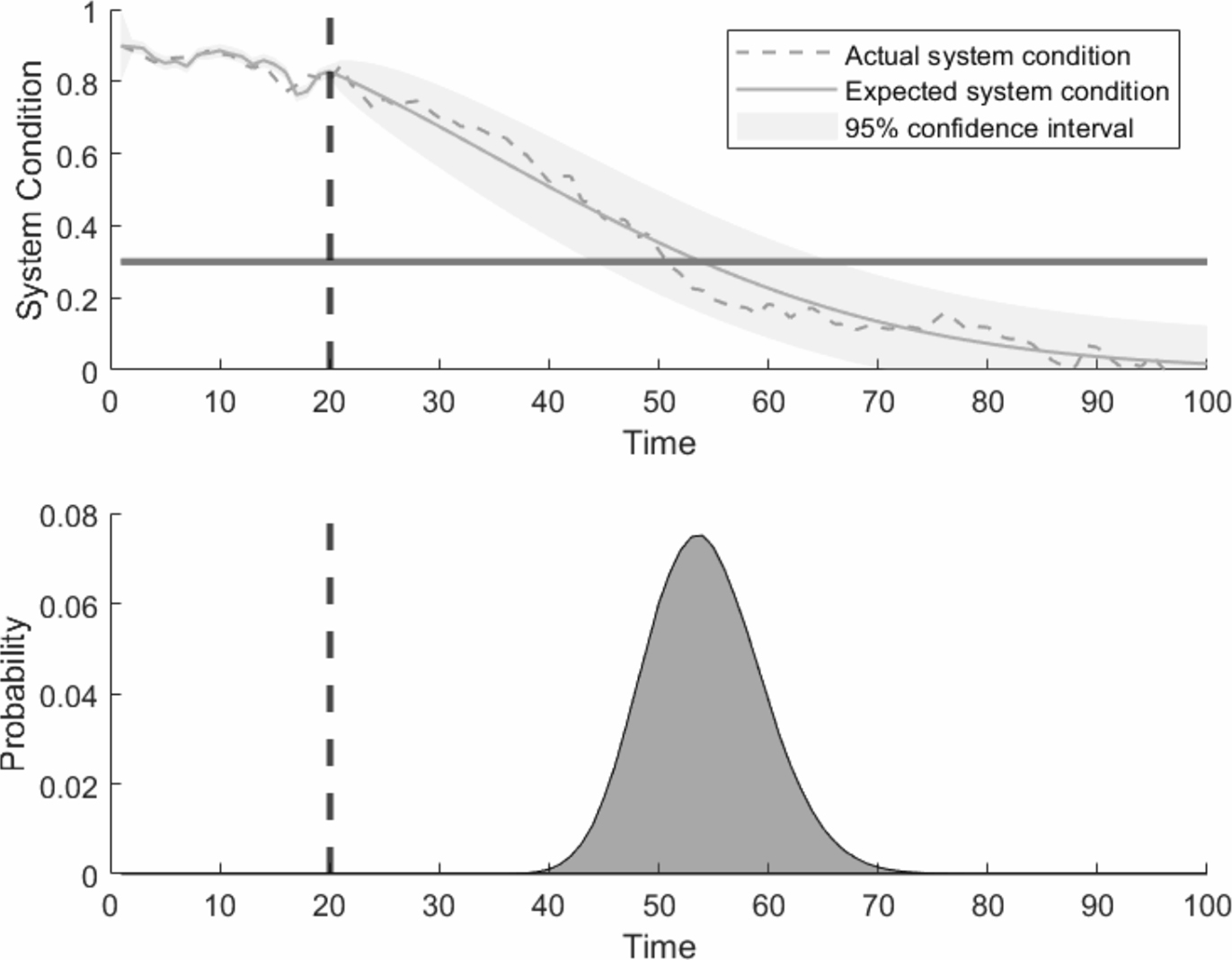
Figure 3.4: Failure time calculation using a random walk (Monte Carlo simulations) approach.
The failure region is defined by fixing the threshold value x̄ = 0.3 in arbitrary units.
According to the results, we can expect a failure time at about 55 seconds (which can be visually obtained just by looking at the area of higher probability content in the PDF at Figure 3.4), which approximately coincides with the time where the real system gets into the failure domain. This simple example reveals the potential of the methodology presented in this chapter for important engineering applications such as failure time estimation.
3.4 Summary
This chapter presented a methodology for damage prognostics and time to failure estimation based on rigorous probabilistic Bayesian principles. First, an architecture for prognostics was developed; in this architecture, the prognostics problem was broken down into two important problems, namely, the sequential state estimation problem and the future state prediction. Since prognostics deals with the prediction of future events, a key feature of the above methodology was a systematic treatment of the various sources of uncertainty. In this sense, the Bayesian framework on which the presented methodology is grounded has shown to be extremely suitable to treat these uncertainties. It was illustrated that, in order to accurately calculate the probability distribution of the time of failure, the prediction needs to be posed as an uncertainty propagation problem that can be solved using a variety of statistical techniques. Some of these methods were briefly discussed, and algorithms were provided for both state estimation and time to failure prediction.