
Chapter 19
Monitoring Project Performance with Earned Value Management
IN THIS CHAPTER
![]() Tracking the terms and formulas that go with earned value management
Tracking the terms and formulas that go with earned value management
![]() Putting earned value management to use with your project
Putting earned value management to use with your project
![]() Estimating an activity’s earned value
Estimating an activity’s earned value
Because you’re reading this chapter, we assume you’re looking for a way to assess your ongoing project performance. Earned value management (EVM), also called earned value analysis (EVA), is a technique that helps determine your project’s schedule status and cost status from your resource expenditures alone. EVM is particularly useful for identifying potential problems on larger projects.
To get the most from this chapter, you need to have some prior experience or knowledge in project management. Here, we help you better understand EVM by defining it, discussing how to determine and interpret variances, and showing you how to use it in your project.
Defining Earned Value Management
Monitoring your project’s performance involves determining whether you’re on, ahead of, or behind schedule and on, under, or over budget. But just comparing your actual expenditures with your budget can’t tell you whether you’re on, under, or over budget — this is where EVM comes in. In this section, we discuss the basics of EVM and the steps involved in conducting an EVM analysis to determine your project’s schedule and cost performance.
Getting to know EVM terms and formulas
Suppose you’re three months into your project and you’ve spent $50,000. According to your plan, you shouldn’t have spent $50,000 until the end of the fourth month of your project. You appear to be over budget at this point, but you can’t tell for sure. Either of the following situations may have produced these results:
- You may have performed all the scheduled work but paid more than you expected to for it — which means you’re on schedule but over budget (not a good situation).
- You may have performed more work than you scheduled but paid exactly what you expected to for it — which means you’re on budget and ahead of schedule (a good situation).
In fact, many other situations may also have produced these same results, but you probably don’t have the time or the motivation to go through each possible situation to figure out which one matches yours. That’s where EVM comes in handy. Evaluating your project’s performance using EVM can tell you how much of the difference between planned and actual expenditures is the result of under- or overspending and how much is the result of performing the project work faster or slower than planned. In the following sections, we review some key terms and formulas you need to know to use EVM.
Spelling out some important terms
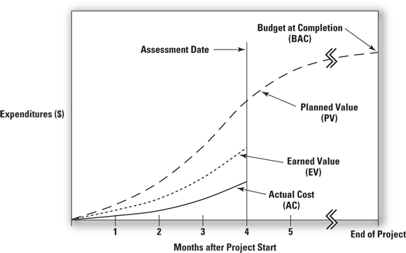
The basic premise of EVM is that the value of a piece of work is equal to the amount of funds budgeted to complete it. As part of EVM, you use the following information to assess your schedule and cost performance throughout your project (see Figure 19-1 for an example):
- Planned value (PV): The approved budget for the work scheduled to be completed by a specified date, also referred to as the budgeted cost of work scheduled (BCWS). The total PV of a task is equal to the task’s budget at completion (BAC) — the total amount budgeted for the task.
- Earned value (EV): The approved budget for the work actually completed by the specified date, also referred to as the budgeted cost of work performed (BCWP).
- Actual cost (AC): The costs actually incurred for the work completed by the specified date, also referred to as the actual cost of work performed (ACWP).
© John Wiley & Sons, Inc.
FIGURE 19-1: Monitoring planned value, earned value, and actual cost.
Use the following indicators to describe your project’s schedule and cost performance with EVM:
- Schedule variance (SV): The difference between the amounts of time budgeted for the work you actually did and for the work you planned to do. The SV shows whether and by how much your work is ahead of or behind your approved schedule.
- Cost variance (CV): The difference between the amount budgeted and the amount actually spent for the work performed. The CV shows whether and by how much you’re under or over your approved budget.
- Schedule performance index (SPI): The ratio of the approved budget for the work performed to the approved budget for the work planned. The SPI reflects the relative amount the project is ahead of or behind schedule, sometimes referred to as the project’s schedule efficiency. You can use the SPI-to-date to forecast the schedule performance for the remainder of the task.
- Cost performance index (CPI): The ratio of the approved budget for work performed to what you actually spent for the work. The CPI reflects the relative value of work done compared to the amount paid for it, sometimes referred to as the project’s cost efficiency. You can use the CPI-to-date to forecast the cost performance for the remainder of the task.
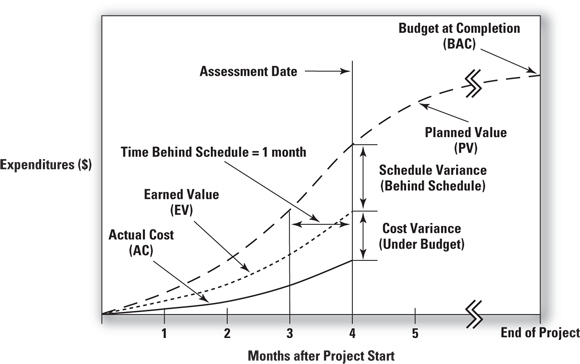
Figure 19-2 shows the key information in an EVM analysis. In this figure, the difference between planned and actual expenditures up to the date of the report is the result of both a schedule delay and cost savings. You can approximate the amount of time you’re behind or ahead of the approved schedule by drawing a line from the intersection of the EV and assessment date lines parallel to the x-axis to the PV line. Doing so in Figure 19-2 suggests that the project being described by the graph is about one month behind schedule.
© John Wiley & Sons, Inc.
FIGURE 19-2: EVM performance indicators.
Defining the formulas of EVM performance descriptors
 Use the following formulas to mathematically define schedule and cost variances and performance indicators:
Tables 19-1 and 19-2 illustrate that a positive variance, or a performance index greater than 1.0, indicates something desirable (that is, you’re either under budget or ahead of schedule, or both) and a negative variance, or a performance index less than 1.0, indicates something undesirable (you’re either over budget or behind schedule, or both!).
TABLE 19-1 Interpretations of Cost and Schedule Variances
Variance | Negative | Zero | Positive |
|---|---|---|---|
Schedule (SV) | Behind schedule | On schedule | Ahead of schedule |
Cost (CV) | Over budget | On budget | Under budget |
TABLE 19-2 Interpretations of Cost and Schedule Performance Indexes
Index | Less than 1.0 | 1.0 | Greater than 1.0 |
|---|---|---|---|
Schedule (SPI) | Behind schedule | On schedule | Ahead of schedule |
Cost (CPI) | Over budget | On budget | Under budget |
Last but not least: Projecting total expenditures at completion
The final step when assessing task performance to date is to update what you expect your total expenditures to be upon task completion. Specifically, you want to determine the following:
- Estimate at completion (EAC): Your estimate today of the total cost of the task
- Estimate to complete (ETC): Your estimate of the amount of funds required to complete all work still remaining to be done on the task
You can use the following two approaches to calculate the EAC:
- Method 1: Assume that the cost performance for the remainder of the task will revert to what was originally budgeted.

- Method 2: Assume that the cost performance for the remainder of the task will be the same as what it has been for the work done to date.

Whether you use Method 1 or Method 2 to calculate EAC, ETC is determined as follows:
Looking at a simple example
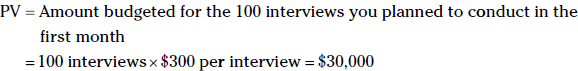
The terms and definitions associated with EVM (see the preceding section) are easier to understand when you consider an example. Suppose you’re planning to conduct a series of telephone interviews. Your interview guide is ready, and each phone interview is independent of the others. You state the following in your project plan:
- Your project will last ten months.
- You will conduct 100 interviews each month.
- You will spend $300 to conduct each interview.
- Your total project budget is $300,000.
During your first month, you do the following:
- Conduct 75 interviews.
- Spend a total of $15,000.
Because you planned to conduct 100 interviews in the first month and you conducted only 75, you’re behind schedule. But because you planned to spend $300 per interview and you spent only $200 (![]() ), you’re under budget. To calculate and then interpret the EVM information associated with this example, follow these steps:
), you’re under budget. To calculate and then interpret the EVM information associated with this example, follow these steps:
- Determine the planned value (PV), earned value (EV), and actual costs (AC) for the month as follows:


- Determine your schedule variance (SV), cost variance (CV), schedule performance index (SPI), and cost performance index (CPI) for the month as follows:

The SPI and CPI make sense when you look at the actual numbers for the month. You originally planned to conduct 100 interviews in the first month, but you finished only 75, which means you accomplished 0.75 of the work scheduled for the month, just as the SPI indicates.
You originally planned to spend $300 per interview, but in the first month you spent only $200 per interview ($15,000 in actual costs ÷ 75 interviews conducted). So for the interviews conducted in the first month, you received a benefit equal to 1.50 times the money you spent, just as the CPI indicates.
Finally, you calculate your revised estimate at completion (EAC) as follows:
- Method 1: Assume that the remaining work is performed at the originally budgeted rate.

If you keep the $7,500 cost savings from the 75 interviews performed in the first month and do the remaining 925 interviews for the $300 per interview originally budgeted, you’ll spend $292,500 to do the 1,000 interviews.
- Method 2: Assume that the remaining work is performed at the same CPI as the work performed to date.

In other words, if you continue to perform your interviews for $200 each rather than the planned $300 each, you’ll spend two-thirds of your total planned budget to complete all 1,000 interviews.
Although you don’t need a formal EVM analysis on a project this simple, in a project with 50 to 100 activities or more, an EVM analysis can help identify general trends in your project’s cost and schedule performances. The earlier you identify such trends, the more easily you can address them when necessary.
Determining the reasons for observed variances
Positive or negative cost or schedule variances indicate that your project performance isn’t going exactly as you planned. After you determine that a variance exists, you need to figure out what’s causing it so you can take corrective actions (if the variance is negative) or continue what you’ve been doing (if the variance is positive).
Possible reasons for positive or negative cost variances include the following:
- Your project requires more or less work to complete a task than you originally planned.
- Work outside the approved scope was performed.
- The people performing the work are more or less productive than planned.
- The actual unit costs of labor or materials are more or less than planned.
- Resources used on other projects were incorrectly recorded to your project, or resources from your project were incorrectly recorded to other projects.
- Actual organization indirect rates are higher or lower than you originally planned (see Chapter 9 for a discussion of indirect rates and the effect they can have on your project expenditures).
Possible reasons for positive or negative schedule variances include the following:
- Work is running ahead of or behind schedule.
- The project requires more or less work than you originally planned.
- People performing the work are more or less productive than planned.
The How-To: Applying Earned Value Management to Your Project
If your project is fairly complex, you may consider using EVM to help control performance. By providing cost and schedule performance assessments of both the total project and its major parts, EVM allows you to identify the likely problem areas so you can take the most effective corrective actions.
The following example presents a more realistic illustration of how EVM can support insightful analysis of your project’s performance.
Suppose the Acme Engineering Company has awarded a contract for the production of two specialized and complex prototypes to Specialized Machinery Corp. The contract calls for Specialized to produce 500 units of Prototype A and 1,000 units of Prototype B. It further states that Specialized will produce Prototype A at the rate of 100 per month and Prototype B at the rate of 250 per month. Production of Prototype A is to start on January 1, and production of Prototype B is to start on February 1. The total budget for the project is $200,000, with $100,000 for Prototype A and $100,000 for Prototype B.
Table 19-3 depicts the project plan.
TABLE 19-3 Plan for Specialized to Produce Prototypes A and B
Activity | Start | End | Elapsed Time | Number of Units | Total Cost |
|---|---|---|---|---|---|
Prototype A | Jan 1 | May 31 | 5 months | 500 | $100,000 |
Prototype B | Feb 1 | May 31 | 4 months | 1,000 | $100,000 |
Total | $200,000 |
Suppose it’s the end of March, and you’re three months into the project. Table 19-4 presents what has happened as of March 31.
TABLE 19-4 Project Status as of March 31
Activity | Start | Elapsed Time | Number of Units Produced | Total Cost |
|---|---|---|---|---|
Prototype A | Jan 1 | 3 months | 150 | $45,000 |
Prototype B | Feb 1 | 2 months | 600 | $30,000 |
Total | $75,000 |
Your job is to figure out your schedule and cost performances to date and to update your forecast of the total amount you’ll spend for both prototypes. Follow these steps:
Determine the planned value (PV), earned value (EV), and actual cost (AC) for Prototype A through March 31 as follows:
PV = $200 per prototype × 100 prototypes per month × 3 months = $60,000
EV = $200 per prototype × 150 prototypes = $30,000
AC = $45,000
Determine the schedule variance (SV), cost variance (CV), schedule performance index (SPI), and cost performance index (CPI) for the production of Prototype A through March 31 as follows:
SV = EV – PV = $30,000 - $60,000 = -$30,000
CV = EV – AC = $30,000 - $45,000 = -$15,000
SPI = EV ÷ PV = $30,000 ÷ $60,000 = 0.50
CPI = EV ÷ AC = $30,000 ÷ $45,000 = 0.67
Your analysis reveals that you produced only half of the copies of Prototype A you thought you would and that each prototype cost you 1.5 times the amount you had planned to spend (1 ÷ CPI =1 ÷0.67 = 1.5; also, the following):

Determine the planned value (PV), earned value (EV), and actual cost (AC) for Prototype B through March 31 as follows:
PV = $100 per prototype × 250 prototypes per month × 2 months = $50,000
EV = $100 per prototype × 600 prototypes = $60,000
AC = $30,000
Determine the schedule variance (SV), cost variance (CV), schedule performance index (SPI), and cost performance index (CPI) for the production of Prototype B through March 31 as follows:
SV = EV – PV = $60,000 - $50,000 = $10,000
CV = EV – AC = $60,000 - $30,000 = $30,000
SPI = EV ÷ PV = $60,000 ÷ $50,000 = 1.20
CPI = EV ÷ AC = $60,000 ÷ $30,000 = 2.00
Your analysis reveals that production of Prototype B is 20 percent ahead of schedule and 50 percent under budget (1 ÷ CPI = 1 ÷ 2 = 0.5; also, [$30,000 expended ÷ 600 prototypes produced] ÷ $100 per prototype = 50 ÷ 100 = 0.5)
Forecast the estimate at completion (EAC) for Prototype A.
Method 1: Assume the remaining work is performed at the originally budgeted rate.
EAC = BAC + AC – EV = $100,000 + $45,000 - $30,000 = $115,000
Method 2: Assume the remaining work is performed at the same CPI as the work performed to date.
EAC = BAC ÷ Cumulative CPI = $100,000 ÷ 0.67 = $150,000
In other words, if the remaining 350 units of Prototype A are produced for the originally planned unit cost of $200, the total cost to produce the full 500 units will be $115,000. If the remaining 350 units of Prototype A are produced for the same $300 unit cost as the first 150, the total cost to produce all 500 will be $150,000.
Forecast the estimate at completion (EAC) for Prototype B.
Method 1: Assume the remaining work is performed at the originally budgeted rate.
EAC = BAC + AC – EV = $100,000 + $30,000 - $60,000 = $70,000
Method 2: Assume the remaining work is performed at the same CPI as the work performed to date.
EAC = BAC ÷ Cumulative CPI = $100,000 ÷ 2.00 = $50,000
In other words, if the remaining 400 units of Prototype B are produced for the originally planned unit cost of $100, the total cost to produce the full 1,000 units will be $70,000. If the remaining 400 units of Prototype B are produced for the same $50 unit cost as the first 600, the total cost to produce all 1,000 will be $50,000.
Determine the overall status of your project by adding together the schedule variances (SV), the cost variances (CV), and the updated estimates at completion (EAC) for Prototypes A and B.
Project SV = -$30,000 + $10,000 = -$20,000
Project CV = -$15,000 + $30,000 = $15,000
Method 1: Assume the remaining work is performed at the originally budgeted rate.
EAC = $115,000 + $70,000 = $185,000
Method 2: Assume the remaining work is performed at the same CPI as the work performed to date.
EAC for the project = $150,000 + $50,000 = $200,000
Table 19-5 summarizes this information.
TABLE 19-5 Performance Analysis Summary
Prototype A | Prototype B | Combined | |
|---|---|---|---|
Prototype A | Prototype B | Combined | |
PV | $60,000 | $50,000 | N/A |
EV | $30,000 | $60,000 | N/A |
AC | $45,000 | $30,000 | $75,000 |
SV | –$30,000 | $10,000 | –$20,000 |
CV | –$15,000 | $30,000 | $15,000 |
SPI | 0.50 | 1.20 | N/A |
CPI | 0.67 | 2.00 | N/A |
EAC* | $115,000 | $70,000 | $185,000 |
EAC** | $150,000 | $50,000 | $200,000 |
* Method 1: Remaining work performed at originally budgeted rate
** Method 2: Remaining work performed at same CPI as work performed to date
If project production rates and costs remain the same until all the required prototypes are produced (this is the Method 2 used to develop the EACs):
- You’ll finish on budget. Table 19-5 shows that EAC for the project will be $200,000, the amount originally budgeted for the whole project.
- You’ll finish five months late. Because Prototype A is being produced at only half the anticipated rate, finishing all of them will take twice the time of five months that was originally planned.
Determining a Task’s Earned Value
The key to a meaningful EVM analysis lies in the accuracy of your estimates of EV. To determine EV, you must estimate:
- How much of a task you’ve completed to date
- How much of the task’s total budget you had planned to spend for the amount of work you’ve completed (the present value of the task)
Consider, for example, that in your planning, you determined that the $10,000 budgeted for your task should be spent in direct proportion to the amount of the task completed. Therefore, if the task is 35 percent complete, you should have spent $3,500 (35 percent multiplied by $10,000).
For tasks with separate components, like producing prototypes or assembling and inspecting the prototypes, determining how much of a task you’ve completed (and, how much of the total corresponding task budget you should’ve spent) is straightforward. However, if your task entails an integrated work or thought process with no easily divisible parts (such as designing a prototype), the best you can do is make an educated guess.
Unfortunately, when you base your analysis on guesses rather than factual data, you open yourself up to the possibility that your EVA will produce an incorrect assessment of how much the schedule is ahead or behind the plan or how much your expenditures are under or over budget (due either to a well-intentioned but incorrect estimate of how complete the task is or to the purposeful manipulation of that number).
Suppose your actual costs to date for your task with the $10,000 budget are $4,500. However, you estimate that the task is only 35 percent complete, which means you should have spent $3,500. In other words, it appears you are $1,000 over budget. However, if you want to hide the fact that you’re over budget, you could claim that you rethought your estimate of how complete the task is and realized the task is actually 45 percent complete. This new estimate of percent complete makes it appear that you should have spent $4,500 ($10,000 multiplied by 45 percent) or, in other words, that the task is exactly on budget. You find out the real amount you over- or underspent on the task only when it is 100 percent complete.
You can use one of the three following approaches to estimate the EV in your project, each of which has certain pros and certain cons:
Percent complete method: With this method, EV is defined to be equal to the product of the fraction representing an estimate of the amount of a task that has been completed and the total budget for the task:
EV = Percent of task completed × Total task budget
So, if you estimate you have completed 40 percent of a task that has a total budget of $10,000, your estimate of the EV of that task, using the percent complete method, would be $4,000:
EV = 40% × $10,000 = $4,000
 The percent complete method is potentially the most accurate if you correctly estimate the fraction of the task you have completed. However, because your estimate of that fraction is a subjective judgment rather than an objective measure, this approach is the most vulnerable to errors or purposeful manipulation.
Milestone method: With this method, EV is defined to be equal to zero until you have completed 100 percent of the task, and then it is 100 percent of the total task budget after you have completed it:
EV = 0 if task is less than 100% complete
EV = Total task budget if task is 100% complete
The milestone method is the most conservative and the least accurate. You expect to spend some money while you’re working on the task. However, this method doesn’t allow you to declare EV greater than $0 until you’ve completed the entire task. Therefore, from the time you start to work on the task (and the time when you most likely will start to spend resources on it) until you have completed it, you’ll appear to be over budget.50/50 method: With this method, EV is defined to be zero before you start the task, a constant 50 percent of the total task budget from the time you start it until the time you finish it, and 100 percent of the total task budget after you finish the task:
EV = 0 (if task hasn’t started)
EV = 50% of total task budget (while task is in progress)
EV = Total task budget (if task is 100% complete)
The 50/50 method is a closer approximation to reality than the milestone method because it allows you to declare an EV greater than $0 for at least some of the time you’re performing the task. However, this approximation can inadvertently mask overspending until the milestone is completed.For example, suppose you have a task with a total budget of $10,000, and you plan to spend the money on this task at a uniform rate over the life of the task. That means when the task is 25 percent complete, you should have expended $2,500 ($10,000 multiplied by 25 percent); when the task is 60 percent complete, you should have expended $60,000 ($10,000 multiplied by 60 percent). Now consider that you’re spending at a uniform rate, exactly as you had planned. If you perform an EVA using this $10,000 activity as one of the tasks, suppose you determine the activity is 30 percent complete, and you’ve spent $4,000 to complete 30 percent of a task with a $10,000 budget.
Arguably, you should’ve spent about 30 percent of the total task budget, or $3,000, to complete 30 percent of the work on the task. The EVA makes it appear that you’re $1,000 over budget. However, using the 50/50 method, you estimate the EV to be $5,000 (50 percent of the total budget for the task), which makes it appear that you’re $1,000 under budget.
Once you’ve started to do work on a task, the 50/50 method makes it appear that you are underspending until you’ve spent 50 percent of the original budget for the task and then overspending once you spend any more, because you can’t declare that you’ve spent more than 50 percent of the initial budget for the task until you complete it entirely.
As you can see, both the milestone method and 50/50 method allow you to approximate EV without estimating the portion of a task that’s been completed. Choosing which of the three methods to use for your project requires that you weigh the potential for accuracy against the possibility of subjective data resulting in misleading conclusions.
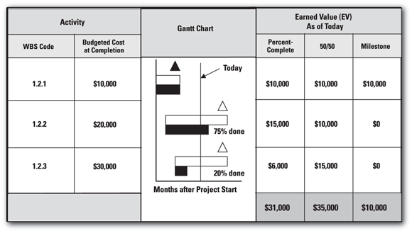
Figure 19-3 compares the accuracy you can achieve when using each of the three different methods in a simple example. Task 1.2, which has a total budget at completion of $60,000, has three subtasks: 1.2.1 (total budget of $10,000), 1.2.2 (total budget of $20,000), and 1.2.3 (total budget of $30,000). Assume that the status of each subtask at the time you’re doing your analysis is as follows:
- Subtask 1.2.1 is 100 percent complete.
- Subtask 1.2.2 is 75 percent complete.
- Subtask 1.2.3 is 20 percent complete.
The EV of Task 1.2 is the sum of the EVs for each of its three subtasks. Using the percent complete method, the EV for subtask 1.2.1 is estimated to be $10,000 ($10,000 multiplied by 100 percent), the EV for subtask 1.2.2 is estimated to be $15,000 ($20,000 multiplied by 75 percent), and the EV for subtask 1.2.3 is estimated to be $6,000 ($30,000 multiplied by 20 percent).
© John Wiley & Sons, Inc.
FIGURE 19-3: Three ways to define earned value.
Using the milestone method, the EV for subtask 1.2.1 is $10,000 because the task is 100 complete, the EV for subtask 1.2.2 is estimated to be $0 because the subtask is less than 100% complete, and the EV for subtask 1.2.3 is estimated to be $0 because the subtask is less than 100 percent complete.
Using the 50/50 method, the EV for subtask 1.2.1 is estimated to be $10,000 because the subtask is 100 percent complete, the EV for subtask 1.2.2 is estimated to be $10,000 ($20,000 multiplied by 50 percent) because the subtask has started, and the EV for subtask 1.2.3 is estimated to be $15,000 ($30,000 multiplied by 50 percent) because the subtask has started.
Finally, the EV for Task 1.2 is determined to be $31,000 ($10,000 + $15,000 + $6,000) with the percent complete method, $10,000 with the milestone method, and $35,000 ($10,000 + $10,000 + $15,000) with the 50/50 method.
 When you use either the milestone method or the 50/50 method, you can improve the accuracy of your EV estimates by defining your lowest-level tasks to be as short as possible, usually completed in two weeks or less (see Chapter 6 for details on how to break down your project with work breakdown structures). When you determine your task status for your progress assessments, most tasks either will not have started or will be finished, thereby increasing the accuracy of your EV estimates.
Relating This Chapter to the PMP Exam and PMBOK 7
Table 19-6 notes topics in this chapter that may be addressed on the Project Management Professional (PMP) certification exam and that are also included in A Guide to the Project Management Body of Knowledge, 7th Edition (PMBOK 7).
TABLE 19-6 Chapter 19 Topics in Relation to the PMP Exam and PMBOK 7
Topic | Location in This Chapter | Location in PMBOK 7 | Comments |
|---|---|---|---|
Definitions of EVM concepts and schedule and cost performance indicators | 2.7.2.3. Baseline Performance 4.4.1. Data Gathering and Analysis | The terms and definitions in this book are the same as those used in PMBOK 7. | |
Updating forecasts of the total task expenditures | 2.7.2.7. Forecasts | The terms and approaches in this book are the same as those used in PMBOK 7. |