
3
Machine Learning: A Key Towards Smart Cyber-Physical Systems
Rashmi Kapoor1*, Chandragiri Radhacharan2 and Sung-ho Hur3
1Department of EEE, VNR VJIET, Hyderabad, India
2Department of EEE, JNTUH University College of Engineering Jagtial, Nachupally (Kondagattu), India
3School of Electronics Engineering, College of IT Engineering, Kyungpook National University, Daegu, South Korea
Abstract
Machine learning is one of the important components of cyber physical systems. Either development or implementation about cloud computing or edge computing, machine learning, deep learning and AI techniques are key to develop a smart cyber physical system. Machine learning has applications in almost all streams of engineering. It is considered as a subset of Artificial Intelligence (AI) but can be seen as an extension of AI that has broadened the application areas of AI.
AI was initiated to make computers mimic human behaviour, considering human to be most intelligent creature on the earth. Although, later when discussions concluded that human behaviour cannot always be considered as intelligent, modified to “mimicking ideal human behaviour”. Modern AI techniques are extracting intelligence not only from human but also from many other creatures like Ant, Bee, Monkey, birds, fishes and many more.
Machine learning added a new feature to AI by trying to make our computer system learn from the data they are receiving. By using Machine Learning techniques, the computers are now not only processing the data, but also extracting the information from that data to give us better results in every next iteration.
Two major thrust research areas in Electrical engineering are Smart Grid and Electric Vehicles. Both these areas are applied to make the power systems and power electronic converters smarter with help of smart inter-disciplinary techniques like machine learning, deep learning, different AI optimization tools etc. So, it is the need of the day for the researchers from different streams to equip themselves with these modern tools.
Machine learning can be applied to various classification applications in electrical engineering like detecting power system faults, transformer faults, machine health monitoring etc. It can also be applied for regression applications like solar radiation prediction, selective harmonic elimination for multi-level inverters, electrical load forecasting etc.
In this chapter basics of machine learning, different machine learning algorithms, stages in machine learning based implementations are discussed. At last Electrical engineering related applications of this mezzanine technology are discussed. Two, end to end applications one in power system and another in power electronics are also covered. Implementation on MATLAB as well as Python platforms are demonstrated through simple examples.
Various Hardware’s that supports machine learning in a cyber-physical system are also discussed and Raspberry-Pi, as a tool for development of machine learning based cyber physical systems is also demonstrated through example.
Keywords: Machine learning, power systems, power electronic converters, MATLAB, python, artificial neural network, artificial intelligence, smart grid
3.1 Introduction
When a computer network, embedded system and physical process are deeply inter-connected to make complete system more efficient, user friendly and/or reliable, such a system is cyber physical system. Smart grid and autonomous vehicles are two main examples of cyber physical systems related to electrical engineering. One of the key components in such systems is artificial intelligence, which adds an extra feature to the system by adding some intelligence to it. The present chapter deals with the basics of Machine learning techniques. Embedding these techniques in a cyber-physical system [20] can make the system intelligent and user friendly.
Artificial Intelligence Techniques [14] are developed to add intelligence to our systems. These techniques extract intelligence from many natural phenomena. Artificial neural networks are evolved by mimicking the structure of human brain, the body part which is responsible for human intelligence. Fuzzy logic is developed by human’s reasoning and decision-making ability. Genetic Algorithm from human evolution system. Ant colony, Particle swam, Bee colony and many other algorithms [1] are developed by mimicking the intelligence in different creatures. The thrust of human to make intelligent machines has led to the development of different algorithms extracting intelligence from different creatures and their behaviour.
One of the main features of intelligence is the “ability to learn”. If this ability to learn can be embedded in our machines that are our computers, it forms a machine learning system. This can be possible only through computer programs that are actual interface between the machine and the human. So, the aim in machine learning is to develop computer programs, that not only process the data to generate output, but also gain information from that data simultaneously, to improve its performance in every next run. For example, if my personal inverter has a computer program, that can learn from data, it may do load scheduling for my home so that battery can last for long duration. Another example can be a microwave, if it also has a machine learning based module, it can learn to predict the cooking time required for a particular item based on the quantity of the food item kept. Personalised house cleaner can be another daily life example, where a computer program can be made to learn from the data. Then, the question may arise about difference between a machine learning algorithm and any other computer program. If your computer program only follows the instruction given, it is not a machine learning program but if along with following instructions it is also learning from experiences (in the form of data), then, it is an intelligent program or can be considered as machine learning, since our machine that is computer is learning with experience like a human. The learning process [13, 15] can be supervised learning [19], unsupervised learning, or reinforcement learning. In case of supervised learning labelled data is available to the machine to learn. In unsupervised learning unlabelled data, it means only input is available to machine to extract some information from it. Whereas in reinforcement learning, unlabelled data with an agent is available for machine to extract fruitful information from the data.
Different applications of Machine learning are divided in some basic streams, like classification, regression, clustering, association, etc. [2]. Classification applications are the cases when the input is kept in one of the two or more predefined classes. The examples of classification applications can be classifying a medical data into healthy and not healthy patient groups or classifying power system voltage and current signals in healthy and faulty power distribution or transmission system. These are the case with binary or two class classification. Similarly, if current and voltages from an electrical distribution system are kept in one of the multiple classes like healthy system, system with LG, LLG, or any other type of fault it became a multi class classification example.
In case of classification applications, the target (or expected outcomes) will be zero and one, if it is a binary classification, or zero, one and two if it is a three-class classification. Thus, the expected outcomes will always be discrete numbers in case of classification applications. Whereas applications like predicting stock market or predicting solar irradiance or electrical loads all will have continuous expected outcome in some range, such applications are regression applications. Although both classification and regression applications come under supervised learning, the type of target data or dependent variable splits them as two different types of applications.
Association and clustering are other applications areas of machine learning that comes under unsupervised learning technique.
3.2 Different Machine Learning Algorithms
Logistic regression is the basic algorithm for classification applications [3], which is based on artificial neural network. Artificial neural network is inspired from human brain or neuron structure. The structure of basic artificial neuron is shown in Figure 3.1(a). Here x1 and x2 represent input to the network, w1 is the weight for connection from input 1 to neuron whereas w2 is weight for connection from input 2 to neuron. So now weighted inputs that are x1 ∗ w1 and x2 ∗ w2, will reach the artificial neuron, where it will first cross through a summation block. Then, this summation output represented by Z in the figure will be acted upon by a function called activation function, to generate the output of the artificial neuron. For logistic regression [18], this function is usually a sigmoidal activation, shown in Figure 3.1(b). This algorithm is suited for binary or two class classification problems. If output of the neuron is close to zero (<0.5), input belongs to one class, if it close to 1 (>0.5), input belongs to other class. Thus z = 0 becomes the partitioning line equation between the two classes. The equation of this partitioning line depends on value of weights w1 and w2. Finding the correct value of w1 and w2 (may be w3, w4… depending upon number of inputs) is the training process. By using large data set of input and output, the optimal values of weights are determined, which gives correct partitioning line between the two classes, so that any new data point can be placed in one of the two classes. The line partitioning will be useful only if, the data to be classified are linearly separable, for linearly non separable data polynomial classification is required by using multi-layer networks. If logistic regression algorithm is required to be used for multiclass classification [6], then OVR (one vs rest) technique can be used. But mostly for multiclass classification problems the sigmoidal activation is replaced by soft-max function and cross entropy loss function is used for training the network.
K nearest neighbor and decision tree [5, 6] are the two non-parametric methods that can be used for classification as well as regression applications. For classification applications, K nearest neighbor determines its ‘k’ nearest neighbors (k = 5, case shown in Figure 3.1(c)), to the unknown data point from the training set and by voting among those ‘k’ neighbors the class of unknown data point is estimated. Various distance formulas are used to find nearest neighbors like Euclidean distance, hamming distance, Manhattan distance, etc. choosing the correct value of ‘k’ is very important for performance of this algorithm.
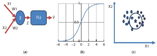
Figure 3.1 (a) Structure of basic artificial neuron, (b) sigmoidal activation function and (c) K nearest neighbor classifier.
Decision tree method is a hierarchical model-based method [2, 3, 5], where we traverse from root node to terminal or leaf node through various branches and nodes. The splitting of branches from nodes is done through feature at that node. The leaf node determines the class of unknown input in case of classification applications, whereas output value, in case of regression applications.
Linear regression is the basic regression algorithm [5, 6] in machine learning, which is again an artificial neural network approach, but instead of sigmoidal activation function as in logistic regression, now the activation function would be linear activation function. Since activation function is linear, the output is not limited between 0 and 1, it can be any value, based on learning parameters. Support vector machine [6, 10] (SVM) improves the performance of logistic and linear regression by considering the support vectors. These support vectors help in finding optimal plane or hyper plane for classification applications. They also provide optimal fitting for data points in case of regression applications. The support vectors are the vectors from classification boundary to nearby data points. The example of choosing the optimal classification line is shown in Figure 3.2(a), where center line is the optimal line as its distance from the neighboring training points (support vectors) is largest.
Naïve Bayes algorithm is based on Bayes theorem [2], where probability of the occurrence of an event is calculated if another event has already happened. This algorithm assumes that all the input features or variables are independent to each other and each has equal contribution towards the output. Ensemble machine learning [4] algorithms are advanced machine learning algorithms to boost the performance the algorithms by combining the different basic techniques.
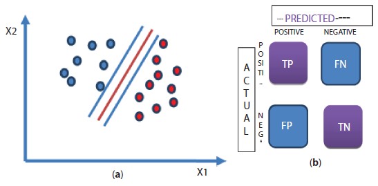
Figure 3.2 (a) SVM Classifier and (b) structure of confusion matrix.
3.2.1 Performance Measures for Machine Learning Algorithms
Performance of any machine learning algorithm is determined by validating its performing on test data. The numerical measure of this performance can be done by different parameters [19, 20]. These parameters will be helpful in comparing different algorithms for a particular application. For classification problems, confusion matrix is one of the important parameters to determine the performance of any algorithm. Confusion matrix is the matrix, that determines how much confused the trained model is, to classify any test point in correct class. The rows of this matrix are actual values, while the columns are predicted output values, for test samples. Figure 3.2(b) shows the confusion matrix for a binary classification problem. The element at first row and first column represented as ‘TP’, i.e., True positive, these are the number of test samples that belongs to positive class and being predicted by the model to be in positive class. So, they are true positive samples. ‘FN’ represent False negative, that are the number of test samples that belongs to positive class but being predicted by the model to be in negative class, so, the negative class prediction by the model is false for these number of samples that is why it is ‘false negative’. Similarly in second row there are ‘false positive’ and ‘true negative’ number of test samples. False negative, are the number of incorrect negative class predictions by the model whereas ‘True positive’ are the number of samples that are correctly predicted by the model to be in negative class. There are many parameters that can be determined from this confusion matrix for comparing different classification algorithms. Some of these parameters are:
Accuracy: Accuracy is defined as ratio of number of correct classifications by the trained model over total number of test samples given to the model.
Precision: It is defined as ratio of number of correct positive class prediction over total positive class predictions made by the model.
Recall/sensitivity: Sensitivity of the model is the number of correct positive class prediction over actual number of positive class samples.
Specificity: Specificity of the model is number of correct negative class prediction over actual number of negative class samples.
F1 score: This parameter summarises Recall and precision by taking harmonic mean of these two parameters.
Trade-off between different parameters needs to be taken base on application requirement, precision may be more important performance criterion for some applications than sensitivity and vice versa.
For regression applications, mean square error, mean absolute error and R2 error or coefficient of determination, are generally used for comparing different algorithms. Mean square error is the mostly used performance measure for regression applications.
3.2.2 Steps to Implement ML Algorithms
The effectiveness of any ML algorithm depends on quantity and quality of data [5, 22]. The first step to implement any ML algorithm is the collection of data. The data can be collected by running the system under different possible conditions and tabulating the input and target variables. Sometimes running actual system under different conditions is not practically feasible, in that case a dummy system model can be developed for collection of data set. Sometimes data collection can be done through a simulated system. But it is essential to validate the simulated data before using it as training data for any implementation. Data can also be downloaded from various online platforms like Kaggle or different government and non-government organizations websites. The next step is to visualize and analyse this raw data, so that any missing or incorrect sample can be corrected or omitted from the data set. Various types of plots are available in MATLAB, Python and R programming platforms available for machine learning implementation that helps in visualization of the data like bar plot, scattered plot, box plot, etc. Different techniques are available to handle missing data if any in the data set. The missing data samples if detected can be ignored or can be predicted from other samples using a machine learning technique. Once the complete data set is available, based on visualization and analysis, features are selected for the model. These featured are independent variables that decide the output of the model. Less number of features may cause under or overfitting of the model, whereas large number of features makes the model complicated and bulky. Once the features are selected, data set is required to be normalized. This step converts the independent variables into zero mean and unit variance, so that all the features get equal dominance towards output determination. Now the data set is ready to be applied to any machine learning algorithm for training. The complete data set is divided in two parts, training set and testing set. The training set is used for training the machine learning model whereas the testing set or validation set is used to validate the performance of the trained model by using various performance measures. Once the best model is achieved, it can be used for inference for unknown data by developing an API or by deploying it on suitable hardware.
3.2.3 Various Platforms Available for Implementation
MATLAB, Python and R programming [12] are the three most popular platforms for implementation of any machine learning based application. All these three provide user friendly instruction set/GUIs for the user. Latest version of MATLAB provides GUI to implement both classification and regression applications that are very good for basic level implementation of any machine learning based application. MATLAB also provides a huge instruction set for programming any machine learning algorithm. Python and ‘R’ are another user-friendly platform that has good number of inbuilt functions for programming any machine learning algorithm very easily.
3.2.4 Applications of Machine Learning in Electrical Engineering
Machine learning can be applied to various electrical engineering applications. Many electrical engineers are working towards development of smart grid, which consists of smart generation, transmission, distribution, and utilization. Machine learning can be an important tool in the development of smart grid. Machine learning based controllers for generators can be developed. Machine learning can also play an important role in increasing the reliability of the electrical grid by developing machine learning based fault detection and isolation systems for different components of the grid like transformer, alternators, and transmission lines. Maintenance of the generating station where human intervention is risky or time consuming can also be done through machine learning. The machine learning based smart loads are already in market like smart air conditioners, air purifiers, washing machines, etc. Artificial intelligence techniques are also playing a role in integrating renewable energy sources with the conventional grid. The forecasting of electrical loads and solar irradiations can be another example where machine learning can be used.
Machine learning also has wide applications in electric vehicle development. Battery health monitoring systems, smart driver assistant system can be developed for electric vehicles using machine learning techniques. Machine learning can also be applied for fault detection and control of various power electronics equipment in the vehicle. For example, dc to dc converters controller and health monitoring system can be developed by using machine learning techniques.
There are various other areas in electrical engineering where machine learning can make the complete system less complicated and more reliable. For example, in electrical drives, safety systems can be developed using machine learning, electrical motor control and health monitoring can also be done using machine learning techniques.
3.3 ML Use-Case in MATLAB
In this section, one example implementation of machine learning algorithms is discussed to classify electrical distribution system line faults. Point of common coupling voltages and neutral current are the independent variables or the input features. The trained machine learning model will be able to classify the system as healthy system or system with LG fault or system with LL faults, etc. The platform demonstrated in this segment is MATLAB. It is a classification application for the machine learning, so different classification algorithms of machine learning can be compared. As discussed, the first step will be to collect dataset for training and testing of different algorithms. Since it is difficult to get huge fault data for any electrical distribution system, either a laboratory dummy model or a simulated distribution system is required to generate different fault condition dataset. In this case, a Simulink model is used to generate PCC voltage and neutral current for different fault cases and healthy power system at different loading conditions. This Simulink scope data will be voltages and current values with corresponding time value. Since it is time-based data, it cannot be directly used as input feature or independent variable for any machine learning model. This time-based data can be converted to time-based features like average value, RMS value or max value etc. This time-based data can also be converted to frequency-based features by using fast Fourier transform or wavelet transform. In the present work fast Fourier transform is used to convert the time-based data to frequency domain and then band power in different frequency ranges based on power spectrum has been chosen to extract features from voltages and current. Seven features are being extracted for each case to complete the data set.
Table 3.1 Sample data set for power system fault classification.
| IN1 | IN2 | IN3 | IN4 | IN5 | IN6 | IN7 | Target |
| 9.00E−05 | 0.002468 | 0.001717 | 200654.5 | 200656.7 | 200666.6 | 1.02E−13 | 0 |
| 0.012805 | 1.341397 | 1.539374 | 0.013685 | 213347.2 | 199668.7 | 224021.9 | 1 |
| 0.960094 | 0.002615 | 0.904782 | 199445.7 | 0.002778 | 213384.6 | 223686.6 | 1 |
| 0.056628 | 0.079739 | 0.026991 | 213557.8 | 199485.2 | 0.028794 | 224088.5 | 1 |
| 0.067671 | 0.082547 | 0.031251 | 42504.31 | 42496.08 | 185594.7 | 579.1227 | 2 |
| 1.939036 | 3.01543 | 2.393509 | 185609.1 | 42495.55 | 42523.11 | 570.2783 | 2 |
| 1.691694 | 1.860545 | 2.426165 | 42622.63 | 185792.5 | 42623.51 | 563.3078 | 2 |
Table 3.1 shows the sample data set extracted for three class classification are: healthy system (target = 0), system with LG fault (target = 1) and system with LL fault (target = 2). Now, features are ready but their distribution is not appropriate, so normalization of data set is required so that it can be in zero mean and unit variance form. The Matlab code for the same is shown in Table 3.2, where each sample is subtracted by mean of its column and divided by standard deviation for the same column. This normalized data set can now be used to train any machine learning classification model.
Table 3.2 Code for data normalization in Matlab.
| for f=1:7 P14(:,f)=(P(:,f)-mean(P(:,f)))/std(P(:,f)) end |
Two cases of implementation can be seen here in MATLAB, first by using GUI app in MATLAB for machine learning that is classification learner application and other by writing an m-file for this implementation.
Let us first see the implementation in classification learner app [16]. This app can be found under APPS tab of MATLAB. After opening the app, clicking on import data will open a new window having three steps as shown in Figure 3.3. The first step is to select the data set from MATLAB workspace. Once data is selected, columns need to be specified as predictor or response in the second step. The predictor means input variables and response means the target value. For this case of classifying the faults, the first seven columns are input features, while the last column is the target output or predictor. In the third step, validation method is selected. Three options available in this step are cross validation, hold out and no validation. In cross validation, data is divided in different parts or folds (the number of folds needs to be specified by the user). One part is kept aside as testing set and remaining parts are used as training set. The performance of the model is evaluated on test set. The complete process is repeated by considering each portion of the data set as test set. This method of validation is particularly suitable for the case when data set is not sufficiently large, as in this case model will be tested on each type of input instead of being tested only on small portion of data. If the data set is sufficiently large the “hold out” validation can be selected in step 3. In this type of validation, a percentage of data is kept aside as testing data for validation of the trained model. The user may also choose ‘no validation’ option in step 3.
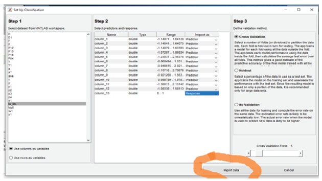
Figure 3.3 Classification learner app in Matlab.
After completing import of data, visualization of data can be done through scattered plot option available in app, and later training can be done by selecting different algorithms and comparing the performance using confusion matrix and ROC curve. The comparison window of various algorithms is also available in the app. The best model can be exported to Matlab workspace for further testing of the model. Once the model is exported simple ‘predict’ command is used to get inferences from the trained machine learning model. The code for the trained machine learning model can also be generated from the classification learner app. This can be easy way to start and understand the machine learning implementation without writing code.
These machine learning models can also be developed by writing an m-file code in MATLAB. Right from importing and handling the data to visualizing the data, MATLAB provides simple inbuilt functions like import, gscatter. MATLAB also provides inbuilt functions for each basic machine learning algorithm, for example, classificationKNN, ClassificationTree, NaiveBayes, svmtrain and svmclassify are some MATLAB functions [17] for K nearest neighbor, decision tree, Naïve Bayes and SVM algorithm, respectively. Matlab also has inbuilt function ‘confusionmat’ for determining confusion matrix, similarly ROC curve and accuracy curves can also be plotted through simple instructions. A simple program for classification using programming in MATLAB is shown in Table 3.4.
Similarly, any regression application where target response is continuous variable can also be implemented in MATLAB either through inbuilt apps or by writing am m-file code. Matlab 2020 which is the latest version has a regression app which is similar to classification learner app that can be used for any regression application if data set is available. Regression applications are based on learning the relation between different independent variables to predict a dependent variable. One simple example can be percentage shortening prediction in stator wingding of induction motor. A machine learning based regression model can be trained to predict the percentage shortening in stator winding with the help of stator current. The steps will be exactly same as what discussed for classification applications; data extraction, data visualization, feature selection, selecting the model, and at last training and testing of algorithm. Data extraction can be done either through a simulation model or from the hardware setup of the system in laboratory. Once data is collected it will be analysed through various visualization tools available, for choosing independent variable or features for the model. The features can be frequency-based features like power spectrum density by performing FFT or wave let transforms. The features can also be sequence component based, that can be obtained by converting three phase stator current to sequence components. Since turn shortening in stator winding causes unbalance in stator winding, so negative or/and zero sequence components can be used for feature extraction. Once features are selected machine learning algorithms can be applied to get a trained model, either through app or by writing a code. A sample regression implementation through Matlab m-file is shown in Table 3.3.
Table 3.3 A sample regression implementation through Matlab m-file.
| load data_regression.mat % loading the data file data1=data_regression(:,2:3) % removing the unwanted columns from data here first column was serial no. so omitted [train_data,test_data ] = holdout(data1,70 );% spilitting the data set as train and test, here 70% for training and 30% for testing In_train=train_data(:,1:end-1); % defining column 1 last-1 as independent variables or input features Tr_train=train_data(:,end);% and last column as response or dependent variable In_test=test_data(:,1:end-1); % for both train and test data set Tr_test=test_data(:,end); N=length(In_train) M=length(In_test) Model1 = fitlm(In_train,Tr_train);% fitlm is inbuilt function for linear regression model training W=Model1.Coefficients{:,1}% to check the trained model parameters %% Mean Square Error predicted_output=predict(Model1,In_test); % applied test inputs to trained model for %prediction mse2=sqrt(mean((predicted_output-Tr_test).^2)) % performance evaluation through mean %square error figure hold on scatter(In_test,Tr_test) % scattered plot for test data set fplot(W(1)+W(2)*x) % plotting the fitted line of the model xlabel({‘Input’}); ylabel({‘output’}); title({‘Regression Using Inbuilt MATLAB Function’}); xlim([-3 3]) hold off |
Table 3.4 A sample Classification implementation through Matlab m-file.
| LR_Model=mnrfit(In_train,Tr_train) % function for multinomial logistic regression % for two class classification ‘fitmodel’ or ‘fitconstrainedmodel’ functions can be used. % testing the trained LR model with new samples that are not used for training Predicted_op = Model.predict(In_test); % to validate the performance the confusion matrix is determined C_matrix = confusionmat(op_test),Predicted_op); knn = ClassificationKNN.fit(In_train,Tr_train,’Distance’,’seuclidean’); % testing the trained KNN model with new samples that are not used for training KNN_predicted = knn.predict(In_test); % to validate the performance the confusion matrix is determined KNN_confusion_Mat = confusionmat(Op_test, KNN_predicted); Op_Nb = NaiveBayes.fit(In_train,Op_train,’Distribution’,dist); % testing the trained Naïve Bayes model with new samples that are not used for training NB_predicted = Nb.predict(In_test); % to validate the performance the confusion matrix is determined NB_confusion_Mat = confusionmat(Op_test, NB_predicted); Svm_Model= svmtrain(In_train,Op_train,’kernel_function’,’rbf ’,’kktviolationlevel’,0.1,’options’,opts); % testing the trained SVM model with new samples that are not used for training Op_svm = svmclassify(Svm_Model, In_test); C_svm = confusionmat(Op_test,Op_svm); |
In the similar way, for any classification application, after loading the classification dataset a code can be written in Matlab. Table 3.4 shows the implementation of different algorithms in an m-file.
3.4 ML Use-Case in Python
Python is a high-level programming language which has a large standard library that facilitated user to complete any complicated task also with small set of instructions or functions. Spyder (scientific python development environment) is an open-source IDE (integrated development environment) to develop and run any python program. The Jupyter notebook is a web-based application where python code along with interactive text based easily sharable notebook can be developed. Pycharm and thonny are other popular IDEs for python. Scikit learn (sklearn) [7, 8, 11] is a machine learning library in python that provides inbuilt functions for various basic machine learning algorithms. Numpy (numerical python) is also a library in python that helps in handling n dimensional arrays. Pandas library in python [8, 9] are used to handle large tabular data sets with labels in a machine learning based program.
Table 3.5 Calling the libraries in python.
| import numpy as np import pandas as pd import matplotlib.pyplot as plt |
To show the implementation of a machine learning classification application, sample data set is generated for power system fault classification as a demonstration. The data is saved as comma separated values (.csv) file, which is loaded in Jupyter notebook. To demonstrate the pandas library data handling, the data set is saved as .csv file and each input column is labeled as I1 to I7 and target column as T.
Before loading the data important libraries need to be called like numpy and pandas for data handling, matplotlib for different plotting functions related to data visualization, error curve plotting, etc. Table 3.5 shows calling of some important python libraries.
Now data set can be loaded using csv_read function available in Pandas. To see some of the initial or ending values of the data “data.head()” or “data.tail()” functions can be used. Pandas library also provides “data. shape” function to find the dimensions of the data set. The complete code for logistic regression and K nearest neighbor algorithm is shown in Table 3.6.
Similarly regression algorithms can also be implemented in python. A sample code is shown in Table 3.7.
Table 3.6 Logistic regression and K nearest neighbor algorithm in python.

Table 3.7 Regression algorithm in python.
| import numpy as np import pandas as pd import matplotlib.pyplot as plt data=pd.read_csv(‘C:/Users/Rashmi_PC/Documents/rashmi_docs/MATLAB/data_regression1.csv’) data.head() X_data1 = data[‘delta’].values y_data1= data[‘percentage shortning’].values from sklearn.linear_model import LinearRegression # LinearRegression function from # # sklearn plt.scatter(x=X_data1,y=y_data1) # library, scattered plot of input data X = np.array(X_data1).reshape(-1, 1) y = np.array(y_data1).reshape(-1, 1) Train_in, Test_in, Train_op, Test_op = train_test_split(X, y, test_size = 0.25) regr = LinearRegression() regr.fit(Train_in, Train_op) print(regr.score(Test_in, Test_op)) out_pred = regr.predict(Test_in) plt.scatter(Test_in, Test_op, color =’b’) plt.plot(Test_in, out_pred, color =’k’) plt.show() |
3.4.1 ML Model Deployment
The process of utilizing trained machine learning model in a cyber-physical system requires deploying the trained machine learning model on suitable hardware that can be embedded in a cyber-physical system. Microcontrollers makes it easier, to include any machine learning algorithm in cyber physical system, thus making it an edge intelligence system.
To load the trained model on a microcontroller it is required to convert the model in embedded C code that can be loaded in a microcontroller. Although it’s not an easy task for everyone to write a machine learning code in embedded C as it does not provide user friendly libraries, to develop a machine learning model. Other easy way is to write a python code for machine learning and deploy that code on raspberry pi, where python libraries can be loaded, and inference can be drawn from the trained model. Raspberry pi, because of hardware limitation, will not be suitable for complex applications. Nvidia provides small portable GPUs like Jetson Nano for fast inferences from large deep learning models. These high-end systems are especially useful for complicated real-time inferences like computer vision applications, or handling time series data using deep neural networks (RNN or LSTM).
3.5 Conclusion
The chapter has given complete basics on machine learning algorithms. The readers can utilize this knowledge to develop their own cyber physical systems for different application areas. Various application areas for electrical engineers to be explored, especially in the field of smart grid and electric vehicles are also discussed. The implementation of basic machine learning algorithms is demonstrated through MATLAB application as well as coding platform and through Python coding.
References
1. Neapolitan, R.E. and Jiang, X., Artificial Intelligence, With an Introduction to Machine Learning, 2nd Edition, United States, CRC Press, 2018.
2. Alpaydın, E., Introduction to Machine Learning, Second Edition, The MIT Press Cambridge, Massachusetts, London, England, 2010.
3. Murphy, K.P., Machine Learning: A Probabilistic Perspective, The MIT Press Cambridge, Massachusetts, London, England, 2012.
4. Zhang, C. and Ma, Y. (Eds.), Computational Intelligence and Complexity, in: Ensemble Machine Learning Methods and Applications, Springer, 2012.
5. Mitchell, T.M., Machine Learning, McGraw-Hill Education, New York, 1997.
6. Mohri, M., Rostamizadeh, A., Talwalkar, A., Foundations of Machine Learning, Second edition, The MIT Press Cambridge, Massachusetts, London, England, 2018.
7. Géron, A., Hands-On Machine Learning with Scikit-Learn and Tensor Flow, 2nd Edition, O’Reilly Media, Inc, September 2019.
8. Sarkar, D., Bali, R., Sharma, T., Practical machine learning with Python, Springer, 2018.
9. Muller, A.C. and Guido, S., Introduction to Machine learning with Python, O’Reilly Media, October 2016.
10. Burkov A. The Hundred-Page Machine Learning Book, 1st ed. Quebec City: Andriy Burkov, 2019.
11. Brownlee, J., Machine Learning Mastery With Python : Understand Your Data, Create Accurate Models and Work Projects End-To-End, Machine Learning Mastery, 2021.
12. Lantz, B., Machine Learning with R, Second Edition, Packt Publishing, July 2015.
13. Simeone, O., A Brief Introduction to Machine Learning for Engineers, 17th, pp. 1–231, now Publishers Inc. Hanover, MA United States May, 2018.
14. Russell, S.J. and Norvig, P., Artificial Intelligence: A Modern Approach, Prentice Hall, Eaglewood Cliffs, New Jersey, 2020.
15. E. Alpaydin, Introduction to Machine Learning, 3rd ed. Cambridge, MA: MIT Press, 2014.
16. Math Works™, https://www.mathworks.com/help/stats/machine-learningin-matlab.html.
17. Paluszek, M. and Thomas, S., MATLAB Machine Learning, Springer, January 2017.
18. Rogers, S. and Girolami, M., A First Course in Machine Learning. CRC Press, London, 2015.
19. Chatterjee, J.M., Kumar, A., Rathore, P.S., Jain, V. (Eds.), Internet of Things and Machine Learning in Agriculture: Technological Impacts and Challenges, vol. 8, Walter de Gruyter GmbH & Co KG, 2021.
20. Vasaki, P., Jhanjhi, N.Z., Humayun., M., Fostering Public-Private Partnership: Between Governments and Technologists in Developing National Cybersecurity Framework, in: Employing Recent Technologies for Improved Digital Governance, pp. 237–255, IGI Global, 2020.
- *Corresponding author: [email protected]