CHAPTER 14
Interest Rate Derivatives
In this chapter we discuss various interest rate derivatives, both commitment and contingent, such as Forward Rate Agreements, Eurodollar Futures, Caps, Floors, Collars, Captions, and Floortions. We also examine callable and putable bonds, which are bonds with built-in interest rate options.
FORWARD RATE AGREEMENTS (FRAs)
A forward rate agreement is a forward contract on an interest rate, such as the six-month LIBOR. Because it is a forward contract, it is traded exclusively over the counter. An FRA represents an agreement between two counterparties to fix a future interest rate. These contracts are cash settled and not delivery settled. There will be a notional principal specified in the agreement, which will be used to compute the terminal cash flow. At maturity, the rate specified in the contract will be invariably different from the prevailing LIBOR. Depending on which is higher, one of the two parties will make a payment to the counterparty. For a potential borrower, the FRA locks in a borrowing rate; for a potential lender, it locks in a lending rate.
In a forward rate agreement, the party who agrees to pay the contract rate is termed the buyer, and the party who agrees to receive the contract rate is termed the seller. Such contracts may be used by hedgers as well as speculators. From a speculative standpoint, traders who are bullish about interest rates will buy FRAs. If the reference rate on the settlement date is higher than the contract rate, then they will receive a cash inflow. If the reference rate is lower, however, then they have to make a cash payment. Similarly, speculators who are bearish about interest rates will sell FRAs. If the reference rate on the settlement date is lower than the contract rate, then they receive a cash inflow. If the reference rate is higher, however, then they have to make a cash payment. We will illustrate this with the help of a numerical example.
An FRA, like all forward contracts, is a commitment contract, and consequently locks in a rate with absolute certainty. Such contracts can also be used to hedge receivables.
An FRA is quoted using two numbers. An ‘A × B’ FRA implies that settlement is A months from today for a loan or deposit of B − A months. The first date is referred to as the settlement date, and the second is termed the final maturity date.
SETTLING AN FRA
Consider a 6 × 12 FRA. Assume that today is 15 March 2021. The spot settlement date is 17 March 2021, assuming a T + 2 settlement cycle. The settlement date will be six months from 17 March 2021. The reference rate will be fixed two days before the settlement date, or six months from the trade date. The maturity date is six months from the settlement date. There are two possibilities: (1) the cash payment may be made on the settlement date, which is termed an in arrears FRA; or (2) the payment may occur on the maturity date, which is termed a delayed settlement FRA.1
Let's assume that the contract rate is 3.6%, and that the LIBOR on the reference fixing date is 3.1%. We will also assume that the notional principal is 12 MM USD, and that the day-count convention is Actual/360.2 Assume that the number of days in the six-month period from settlement until final maturity is 182 days.
Because the contract rate is higher than the reference rate, the buyer has to make a payment. The amount due is:
Had the FRA been a delayed settlement contract, the cash flow would occur six months from the settlement date, and the value on the settlement date would be the present value of this amount, determined by discounting at the LIBOR prevailing on the reference fixing date. In our case, the present value would be

DETERMINING BOUNDS FOR THE FRA RATE
If we are given money market interest rates, we can determine the upper and lower bounds for the FRA rate. Assume that the interest rates in the market are as follows. The lower rate is what the dealer will pay when it borrows, while the higher rate is what it will charge when it lends.
EURODOLLAR FUTURES
Eurodollars are dollars traded outside the borders of the United States. Eurodollar (ED) futures contracts trade on the IMM in Chicago, which is a part of the CME Group. The underlying interest rate is the London Inter Bank Offer Rate (LIBOR). Each futures contract is for a time deposit with a principal of 1 MM and three months to maturity.
The quarterly cycle for Eurodollar contracts is March, June, September, and December. On the CME, a total of 40 quarterly futures contracts spanning 10 years are listed at any point in time. In addition, the four nearest serial months are also listed. Let us assume that we are standing on June 28, 2021. The four serial months that would be available would be July, August, October, and November 2021. The remaining available months would be September 2021; December 2021; March, June, September, and December of 2022–2030; March 2031; and June 2031.
The price of an ED futures contract is quoted in terms of an IMM index, and implies an interest rate.
The implicit interest rate in this case is an actual or add-on interest rate and not a discount rate. Thus, a quoted rate of 3% per annum means that for a 90-day loan with a maturity value of 1 MM, the terminal amount payable or receivable is
CALCULATING PROFITS AND LOSSES ON ED FUTURES
Assume that the futures price is 97.20. This represents a yearly interest rate of 2.8% per annum or 0.70% per quarter. The implied interest amount is
If the futures price were to fall to 96.80 at the end of the day, then it would represent a quarterly interest payment of $8,000 on a deposit of one million.
Consider a person who goes long in an ED futures contract at 97.20. Such a person is agreeing to lend money at the equivalent interest rate, namely 0.70% per quarter. It must be understood that a long position in ED futures means that the investor is willing to make a term deposit of three months. Thus, it is a lender. If interest rates rise subsequently to 3.20% per annum, that is, the futures price goes down to 96.80, and the contract is marked to market, then the long will lose $1,000. The rationale may be understood as follows. When the contract is marked to market, it is as if the dealer is offsetting by going short, which in this case means that it is agreeing to borrow at 3.20% per quarter. Thus, when the interest rates rise the longs will lose, whereas when the interest rates fall the shorts will lose.
This explains the logic behind quoting futures prices in terms of an index, rather than in terms of interest rates. If futures prices were to be quoted in terms of interest rates, then the longs would gain when the futures prices fall and the shorts would gain when the futures prices rise. This is unlike all other futures markets, where the longs gain when futures prices rise, whereas the shorts gain if futures prices fall. Thus, to make money market futures consistent with other futures markets, we do not quote futures prices in terms of interest rates, but do so in terms of an index. When the index rises, the longs will gain; when it falls, the shorts will gain.
A second reason why futures prices are quoted in terms of an index is to ensure that the bid prices are lower than the ask. In practice, for an investor, the borrowing rate will be higher than the lending rate. Thus, if ED futures were to be quoted in terms of interest rates, the bid will be higher than the ask. For the other products on which futures are available, however, the bid is lower than the ask. Consequently, we express futures prices in terms of an index to ensure that the bid is lower than the ask.
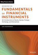
Now consider the case where the ED index changes from F0 to F1. The profit for a long is
The corresponding profit for the short is

LOCKING IN A BORROWING RATE
Now we will illustrate how borrowing and lending rates can be locked in using ED futures.
LOCKING IN A LENDING RATE
Here is an example on how to lock in a lending rate.
ED futures can be used to hedge short-term loans and deposits for periods that are close to 90 days but are not exactly equal to three months. The inherent assumption is that the N day rate, where N is close to 90, is perfectly correlated with the 90-day rate.
The number of contracts required is N/90 per million dollars being hedged. Here is an illustration.
THE NO-ARBITRAGE PRICING EQUATION
We will now state an expression for the futures price, which will preclude both cash-and-carry and reverse cash-and-carry arbitrage, for a given set of interest rates. Let us denote the day on which we are standing as day ‘t.’ The futures contract is assumed to expire at ‘T.’ We will denote the Eurodollar rate for a ‘T − t’ day loan by s1 and the borrowing/lending rate for a ‘T + 90 − t’ day loan by s2.
In order to rule out both forms of arbitrage, we require that

Here is an illustration.
CREATING A FIXED-RATE LOAN
Assume that Rolta Bank is able to borrow money at LIBOR for three-month periods. Consequently, the interest payable on its liability is variable. The bank, however, has a potential client who wishes to borrow at a fixed rate for a period of one year. Thus, the interest receivable from the proposed asset is fixed in nature. The bank would like to use futures contracts to mitigate the risk arising from the fact that it is borrowing at a floating rate but is lending at a fixed rate. It turns out that ED futures contracts can be used to hedge the funding risk and determine a suitable rate that can be quoted by the bank while negotiating a fixed rate loan. We will illustrate the principle involved with the help of an example.
30-YEAR T-BOND FUTURES CONTRACTS
The underlying asset is a T-bond with a face value of $100,000. Multiple grades are allowable for delivery. The deliverable grades must, if they are callable in nature, not be callable for at least 15 years from the first day of the delivery month, and if they are not callable in nature, must have a maturity of at least 15 years from the first day of the delivery month. The actual futures price is subject to a conversion factor. At any point in time, the first three months from the March quarterly cycle will be listed. Thus, on June 29, 2021, the available contracts will be September 2021, December 2021, and March 2022.
All the contracts are subject to delivery settlement.
CONVERSION FACTORS
As one can see from the contract specifications, a wide variety of notes and bonds with different coupons and maturity dates will be eligible for delivery under any particular futures contract. The choice as to which bond to deliver will be made by the short, and obviously the price it receives will depend on the bond that it chooses to deliver. If the short were to deliver a more valuable bond, it should receive more than it would if it had delivered a less valuable bond. Thus, in order to facilitate comparisons between bonds, the exchange specifies a conversion factor for each bond that is eligible for delivery. This is nothing but a multiplicative price adjustment system to facilitate comparisons between different bonds that are eligible for delivery.
The conversion factor for a bond is the value of the bond per $1 of face value, as calculated on the first day of the delivery month, using an annual YTM of 6% with semiannual compounding. For the purpose of calculation, the life of the bond is rounded down to the nearest three months. If, after rounding, the bond were to have a life that is an integer multiple of semiannual periods, then the first coupon will be assumed to be paid after six months. After rounding, however, if the life of the bond were not to be equal to an integer multiple of half-yearly periods, then the first coupon will be assumed to be paid after three months and the accrued interest will be subtracted. The following detailed examples will illustrate these principles.
The Invoice Price, which is the price received by the short, is calculated as follows:

where CFi is the conversion factor of Bond i, F is the quoted futures price per dollar of face value,3 and AIi is the accrued interest.
Why do we adopt two different procedures for calculating the CF? The CF is used to multiply the quoted futures price, which is a clean price. Hence the CF should not include any accrued interest. In the first example, the bond has a life that is an integer multiple of semiannual periods after rounding off. Consequently, we need not be concerned with accrued interest. In the second example, however, accrued interest for a quarter is present in the value we get in the second step. Hence, in this case, we need to subtract this interest in order to arrive at the conversion factor.
INTEREST RATE OPTIONS
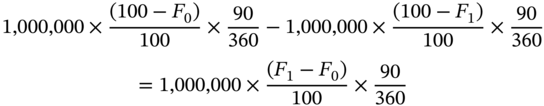
Valuing interest rate options requires us to model the evolution of interest rates over time. Equilibrium models of the interest rate attempt to model the rates using economic variables. The problem in practice is that the bond prices predicted by these models do not match the observed bond prices. An alternative is to take the available term structure and derive an interest rate tree that is consistent with the observed spot rates. For the rest of this chapter we will use a tree derived by calibrating a model known as the Ho-Lee model to a given vector of spot rates (Table 14.1).
STATE PRICES
Arrow-Debreu securities, also known as pure securities, will pay a dollar if a particular state of nature were to occur. In all other states of nature, however, the payoff will be zero. Obviously, each node of a binomial tree represents a particular state of nature. The price at time zero of a pure security that pays off a dollar at a particular node is called the state price of the node. Figure 14.1 depicts the interest rate tree that has been obtained by calibrating the Ho-Lee Model.
TABLE 14.1 Vector of Spot Rates
| Period | Spot Rate |
|---|---|
| 1 | 6.00% |
| 2 | 5.80% |
| 3 | 6.05% |
| 4 | 5.90% |
FIGURE 14.1 No-Arbitrage Interest Rate Tree

FIGURE 14.2 State Price Tree
At a point in time, a security that pays a dollar in all states of nature is a riskless security. The sum of the prices of all the pure securities for a point in time should be equal to the present value of a dollar, discounted at the riskless rate. Consider the two-period spot rate of 5.80% per annum. Figure 14.2 depicts the state price tree corresponding to the interest rate tree that has been derived.

CALLABLE AND PUTABLE BONDS
Consider a two-period bond with a coupon of 8% per annum. The value of this bond is:

Now assume that this bond is callable after a period, and if called, a premium of $15 is payable. The value of the bond at the upper node at time t1 is

If called, the issuer must pay ![]() . Thus, the bond will not be called.
. Thus, the bond will not be called.
The value of the bond at the lower node at time t1 is

If called, the issuer must pay ![]() . Thus, the bond will be called. Hence the value of the callable is $1,046.7846 at the upper node and 1,055 at the lower node. Hence the price at the outset is
. Thus, the bond will be called. Hence the value of the callable is $1,046.7846 at the upper node and 1,055 at the lower node. Hence the price at the outset is
Thus, the value of the call option inherent in the callable bond is
Now consider a putable bond which can be put back at par. Assume the coupon is 6% per annum. The model value at the upper node is

If the bond is put back, the holder will get $1,030. Thus, the bond will be put back. At the tower node the model value is

If the bond is put back, the holder will get 1,030. Thus, the bond will not be put back. Thus, the value of the putable bond at the outset is
Had it been a plain-vanilla bond the value would have been

Thus, the value of the put option inherent in the bond is
CAPS, FLOORS, AND COLLARS
A caplet is a call option on an interest rate, while a floorlet is a put option on an interest rate. Consider a one-period caplet with an exercise price of 5%. Let the underlying principal be $5,000,000. Each time period is assumed to be of six months, duration, and we will take it as 0.5 years in order to avoid issues regarding day-count conventions.
At time t1, the rate may be 6.5983% or 4.5983%. In the first case the caplet will be in the money, whereas in the second case it will be out of the money. The payoff, if it is in the money, is
In the case of interest rate options, the payoff will occur not when the option expires, but at a point in time when the next interest payment is due. In the above case, the rate as determined at t1 is applicable for computing the interest due at t2. Consequently, the caplet will pay off at t2.
Thus, the value of the caplet at time t0 may be computed as:

A floorlet is a put option on an interest rate. Let us consider a floorlet with the same exercise price and underlying principal as the caplet. The payoff will be zero if the interest rate is 6.5983%, as the option will be out of the money; however, there will be a positive payoff at state if the rate is 4.5983, which is given by:
This payoff will obviously occur at time t2. Consequently, the value of the floorlet at t0 is:

A cap is a portfolio of caplets that can be acquired by a borrower who has availed itself of a floating-rate loan in order to protect against an increase in interest rates. Similarly, a floor is a portfolio of floorlets that can be acquired by a lender who has made a loan on a floating-rate basis to protect itself against a decline in interest rates. An interest rate collar is a combination of a cap and a floor. It requires the investor to take a long position in a cap and a short position in a floor.
CAPTIONS AND FLOORTIONS
A caption is a financial instrument that gives the holder the right to buy a cap at a future point in time. Consider a company that is likely to borrow funds at a future point in time. In the event that it takes the loan, the prospect of a high rate of interest would be of concern. Consequently, the company may decide to acquire the cap. If, however, it decides not to take the loan, there is no need to acquire the cap. The caption gives the potential borrower the ability to lock in a contract rate in advance for the cap, without taking away its freedom to refrain from exercise if the loan is not taken. If the contract rate in the option is X and prevailing reference rate in the future is K, the caption is exercised if K > X. Otherwise, the buyer can allow the caption to expire and acquire a cap at the prevailing contract rate, if it decides to take the loan. In the event of the loan not being availed of, the cap need not be exercised.
Similarly, a floortion gives the holder the right to buy a floor at a future point in time. An entity that is likely to make a loan at a future point in time may be interested in such an instrument. A potential lender would be perturbed by the prospect of declining interest rates. If it acquires a floortion, it can exercise if the option is in the money; otherwise, the floortion can be allowed to expire. If the lender decides not to extend the loan, the option can be allowed to expire unexercised. If the contract rate of the floortion is X, and prevailing reference rate in the future is K, the floortion will be exercised if X > K. Otherwise, it will be allowed to expire.
NOTES
- 1 See Chance (2001).
- 2 For contracts in USD and EUR, the day-count convention is Actual/360, as is the practice in the money market. For transactions in GBP, AUD, CAD, or JPY, the convention is Actual/365.
- 3 T-Bond futures prices are quoted in the same way as the cash market prices; that is, they are clean prices.