
Chapter 1
Leveraging Ensembles of Learners
IN THIS CHAPTER
![]() Considering decision trees
Considering decision trees
![]() Performing predictions
Performing predictions
![]() Using gradient descent
Using gradient descent
![]() Working with multiple predictors
Working with multiple predictors
After discovering so many complex and powerful algorithms, you might be surprised to discover that a summation of simpler machine learning algorithms can often outperform the most sophisticated solutions. Such is the power of ensembles, which are groups of models made to work together to produce better predictions. The amazing thing about ensembles is that they are made up of groups of singularly nonperforming algorithms.
Ensembles don’t work much differently from the collective intelligence of crowds, through which a set of wrong answers, if averaged, provides the right answer. Sir Francis Galton, the British, Victorian-era statistician known for having formulated the idea of correlation, narrated the anecdote of a crowd in a county fair that could guess correctly the weight of an ox after all the people’s previous answers were averaged. You can find similar examples everywhere and easily re-create the experiment by asking friends to guess the number of sweets in a jar and averaging their answers. The more friends who participate in the game, the more precise the averaged answer.
Luck isn’t what’s behind the result; it’s simply the law of large numbers in action (see more at https://www.britannica.com/science/law-of-large-numbers).
Even though an individual has a slim chance of getting the right answer, the guess is better than a random value. By accumulating guesses, the wrong answers tend to distribute themselves around the right one. Opposite wrong answers cancel each other when averaging, leaving the pivotal value around which all answers are distributed, which is the right answer. You can employ such an incredible fact in many practical ways (consensus forecasts in economics and political sciences are examples) and in machine learning.
 You don’t have to type the source code for this chapter manually. In fact, using the downloadable source is a lot easier. The source code for this chapter appears in the
 DSPD_0401_Random_Forests.ipynb source code file for Python and DSPD_R_0401_Random_Forests.ipynb source code file for R. See the Introduction for details on how to find these source files.
Leveraging Decision Trees
Ensembles are based on a recent idea (formulated around 1990), but they leverage older tools, such as decision trees, which have been part of machine learning since 1950. Texts such as Machine Learning For Dummies, by John Paul Mueller and Luca Massaron (Wiley), cover decision trees as simple learners. You can also find an overview of them at https://towardsdatascience.com/decision-trees-in-machine-learning-641b9c4e8052. Decision trees at first looked quite promising and appealing to practitioners because of their ease of use and understanding. After all, a decision tree can easily do the following:
- Handle mixed types of target variables and predictors, with very little or no feature preprocessing (missing values are handled almost automatically)
- Ignore redundant variables and select only the relevant features
- Work out-of-the box, with no complex hyperparameters to fix and tune
- Visualize the prediction process as a set of recursive rules arranged in a tree with branches and leaves, thus offering ease of interpretation
Given the range of positive characteristics, you may wonder why practitioners slowly started distrusting decision trees after a few years. The main reason is that the resulting models often have high variance in the estimates.
To grasp the critical problem of decision trees better, you can consider the problem visually. Think of the tricky situation of the bull's-eye problem that requires a machine learning algorithm to approximate nonlinear functions (as neural networks do) or to transform the feature space (as when using a linear model with polynomial expansion or kernel functions in support vector machines). Figure 1-1 shows the squared decision boundary of a single decision tree (on the left) as compared to an ensemble of decision trees (on the right).
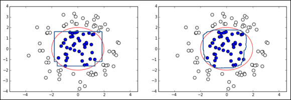
FIGURE 1-1: Comparing a single decision tree output to an ensemble of decision trees.
Decision trees partition the feature space into boxes and then use the boxes for classification or regression purposes. When the decision boundary that separates classes in a bull’s-eye problem is an ellipse, decision trees can approximate it by using a certain number of boxes.
The visual example seems to make sense and might give you confidence when you see the examples placed far from the decision boundary. However, in proximity of the boundary, things are quite different from how they appear. The decision boundary of the decision tree is very imprecise, and its shape is extremely rough and squared. The issue is visible on bidimensional problems. It decisively worsens both as feature dimensions increase and when in the presence of noisy observations (observations that are somehow randomly scattered around the feature space). You can improve decision trees using some interesting heuristics that stabilize results from trees:
- Keep only the correctly predicted cases to retrain the algorithm.
- Build separate trees for misclassified examples.
- Simplify trees by pruning the less decisive rules.
Apart from these heuristics, the best trick is to build multiple trees using different samples and then compare and average their results. The example in Figure 1-1, shown previously, indicates that the benefit is immediately visible. As you build more trees, the decision boundary gets smoother, slowly resembling the hypothetical target shape.
Growing a forest of trees
Improving a decision tree by replicating it many times and averaging results to get a more general solution sounded like such a good idea that it spread, and practitioners created various solutions. When the problem is a regression, the technique averages results from the ensemble. However, when the trees deal with a classification task, the technique can use the ensemble as a voting system, choosing the most frequent response class as an output for all its replications.
 When using an ensemble for regression, the standard deviation, calculated from all the ensemble’s estimates for an example, can give you an estimate of how confident you can be about the prediction. The standard deviation shows how good a mean is. For classification problems, the percentage of trees predicting a certain class is indicative of the level of confidence in the prediction, but you can’t use it as a probability estimate because it’s the outcome of a voting system.
Deciding on how to compute the solution of an ensemble happened quickly; finding the best way to replicate the trees in an ensemble required more research and reflection. The first solution is pasting, that is, sampling a portion of your training set. Initially proposed by Leo Breiman, pasting reduces the number of training examples, which can become a problem for learning from complex data. It shows its usefulness by reducing the learning sample noise (sampling fewer examples reduces the number of outliers and anomalous cases). After pasting, Professor Breiman also tested the effects of bootstrap sampling (sampling with replacement), which not only leaves out some noise (when you bootstrap, on average you leave out 37 percent of your initial example set) but also, thanks to sampling repetition, creates more variation in the ensembles, improving the results. This technique is called bagging (also known as bootstrap aggregation).
Bootstrapping is one of the validation alternatives. It’s a method long used to estimate the sampling distribution of statistics, which are presumed not to follow a previously assumed distribution. Bootstrapping works by building a number (the more the better) of samples of size n (the original in-sample size) drawn with repetition. To draw with repetition means that the process could draw an example multiple times to use it as part of the bootstrapping resampling. Bootstrapping has the advantage of offering a simple and effective way to estimate the true error measure. In fact, bootstrapped error measurements usually have much less variance than cross-validation ones. On the other hand, validation becomes more complicated because of the sampling with replacement, so your validation sample comes from the out-of-bootstrap examples. Moreover, using some training samples repeatedly can lead to a certain bias in the models built with bootstrapping.
Breiman noticed that results of an ensemble of trees improved when the trees differ significantly from each other (statistically, they’re uncorrelated), which leads to the last technique transformation: sampling from the training features. This technique allows for the creation of mostly uncorrelated ensembles of trees. The approach performs predictions better than bagging. The transformation tweak samples both features and examples. Breiman, in collaboration with Adele Cutler, named the new ensemble Random Forests (RF).
Random Forests is a trademark of Leo Breiman and Adele Cutler (see https://www.stat.berkeley.edu/~breiman/RandomForests/). For this reason, open source implementations often have different names, such as randomForest in R (see https://www.rdocumentation.org/packages/randomForest/versions/4.6-14/topics/randomForest) or RandomForestClassifier in Python’s Scikit-learn (see https://scikit-learn.org/stable/modules/generated/sklearn.ensemble.RandomForestClassifier.html).
RF is a classification (naturally multiclass) and regression algorithm that uses a large number of decision tree models built on different sets of bootstrapped examples and subsampled features. Its creator strove to make the algorithm easy to use (little preprocessing and few hyperparameters to try) and understandable (the decision tree basis) that can democratize the access of machine learning to nonexperts. In other words, because of its simplicity and immediate usage, RF can allow anyone to apply machine learning successfully. The algorithm works through a few repeated steps:
- Bootstrap the training set multiple times. The algorithm obtains a new set to use to build a single tree in the ensemble during each bootstrap.
- Randomly pick a partial feature selection in the training set to use for finding the best split variable every time you split the sample in a tree.
- Create a complete tree using the bootstrapped examples. Evaluate new subsampled features at each split. Don’t limit the full tree expansion to allow the algorithm to work better.
- Compute the performance of each tree using examples you didn’t choose in the bootstrap phase (out-of-bag estimates, or OOB). OOB examples provide performance metrics without cross-validation or using a test set (equivalent to out-of-sample).
- Produce feature importance statistics and compute how examples associate in the tree’s terminal nodes.
- Compute an average or a vote on new examples when you complete all the trees in the ensemble. Declare for each of them the average estimate or the winning class as a prediction.
All these steps reduce both the bias and the variance of the final solution because the solution limits the bias. The solution builds each tree to its maximum possible extension, thus allowing a fine fitting of even complex target functions, which means that each tree is different from the others. It’s not just a matter of building on different bootstrapped example sets: Each split taken by a tree is strongly randomized, meaning that the solution considers only a random feature selection. Consequently, even if an important feature dominates the others in terms of predictive power, the times a tree doesn’t contain the selection allows the tree to find different ways of developing its branches and terminal leaves.
The main difference with bagging is this opportunity to limit the number of features to consider when splitting the tree branches. If the number of selected features is small, the complete tree will differ from others, thus adding uncorrelated trees to the ensemble. On the other hand, if the selection is small, the bias increases because the fitting power of the tree is limited. As always, determining the right number of features to consider for splitting requires that you use cross-validation or OOB estimate results.
No problem arises in growing a high number of trees in the ensemble. You do need to consider the cost of the computational effort because completing a large ensemble takes a long time. A simple demonstration conveys how an RF algorithm can solve a simple problem using a growing number of trees. Python and R offer good implementations of the algorithm:
- The Python implementation is easier to parallelize.
- The R implementation has more parameters.
Seeing Random Forests in action
Because the test is computationally expensive, the example starts with the Python implementation. This example uses the digits dataset that you use in the previous chapter when challenging a support vector classifier:
import numpy as np
from sklearn import datasets
from sklearn.model_selection import validation_curve
from sklearn.ensemble import RandomForestClassifier
digits = datasets.load_digits()
X,y = digits.data, digits.target
series = [10, 25, 50, 100, 150, 200, 250, 300]
RF = RandomForestClassifier(random_state=101)
train_scores, test_scores = validation_curve(RF,
X, y, 'n_estimators', param_range=series,
cv=10, scoring='accuracy',n_jobs=-1)
The example begins by importing functions and classes from Scikit-learn: numpy, the datasets module, the validation_curve function, and RandomForestClassifier. The last item is Scikit-learn's implementation of RF for classification problems. The validation_curve function is particularly useful for the tests because it returns the cross-validated results of multiple tests performed on ensembles made of differing numbers of trees (similar to learning curves).
The example will build almost 11,000 decision trees. To make the example run faster, the code sets the n_jobs parameter to –1, allowing the algorithm to use all available CPU resources. This setting may not work on some computer configurations, which means setting n_jobs to 1. Everything will work, but the process takes longer.
After completing the computations, the code outputs a plot that reveals how the RF algorithm converges to a good accuracy after building a few trees, as shown in Figure 1-2. It also shows that adding more trees isn't detrimental to the results, although you may see some oscillations in accuracy because of estimate variances that even the ensemble can’t control fully.
import matplotlib.pyplot as plt
%matplotlib inline
plt.figure()
plt.plot(series, np.mean(test_scores,axis=1), '-o')
plt.xlabel('number of trees')
plt.ylabel('accuracy')
plt.grid()
plt.show()
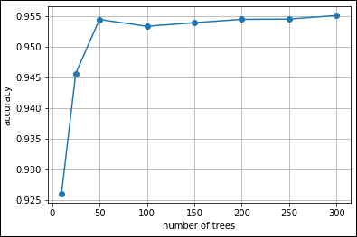
FIGURE 1-2: Seeing the accuracy of ensembles of different sizes.
Understanding the importance measures
Random Forests algorithms have these benefits:
- They fit complex target functions, but have little risk in overfitting.
- They select the features they need automatically (although the random subsampling of features in branch splitting influences the process).
- They are easy to tune up because they have few hyperparameters, and the most important one you should care is often just the number of subsampled features.
- They offer OOB error estimation, saving you from setting up verification by cross-validation or test set.
Note that each tree in the ensemble is independent from the others (after all, they should be uncorrelated), which means that you can build each tree in parallel to the others. Given that all modern computers have multiprocessor and multithread functionality, they can perform computations of many trees at the same time, which is a real advantage of RF over other machine learning algorithms.
An RF ensemble can also provide additional output that could be helpful when learning from data. For example, it can tell you which features are more important than others. You can build trees by optimizing a purity measure (entropy or gini index) so that each split chooses the feature that improves the measure the most. When the tree is complete, you check which features the algorithm uses at each split and sum the improvement when the algorithm uses a feature more than once. When working with an ensemble of trees, simply average the improvements that each feature provides in all the trees. The result shows you the ranking of the most important predictive features.
Practitioners evaluate the importance features in RFs using gini importance, which is also called mean decrease impurity. You can compute it in both Python and R algorithm implementations. Importance estimation that uses mean decrease impurity after building each tree replaces each feature with junk data and records the decrease in predictive power after doing so. If the feature is important, crowding it with casual data harms the prediction, but if it’s irrelevant, the predictions are unchanged. Reporting the average performance decrease in all trees that results from randomly changing the feature is a good indicator of a feature’s importance.
You can use importance output from RFs to select features to use in the RF or in another algorithm, such as a linear regression. The Scikit-learn algorithm version offers a tree-based feature selection, which provides a way to select relevant features using the results from a decision tree or an ensemble of decision trees. You can use this kind of feature selection by employing the SelectFromModel function found in the feature_selection module (see https://scikit-learn.org/stable/modules/generated/sklearn.feature_selection.SelectFromModel.html).
Configuring your system for importance measures with Python
To make the example code work for checking importance measures in Python, you need to install the rfpimp (https://pypi.org/project/rfpimp/) package. The article at https://explained.ai/rf-importance/index.html tells why this particular package is so important. To install the package, you begin by opening an Anaconda Prompt (don't use a standard command prompt or terminal window because neither has the required environmental setup). At the prompt, you type
conda install -c conda-forge rfpimp
and press Enter. The command runs for a while, seemingly doing nothing. However, at some point you see a description of what conda will do, as shown in Figure 1-3. Simply type y and press Enter to install the package.
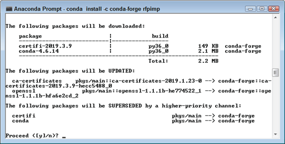
FIGURE 1-3: Installing the rfpimp package in Python.
Seeing importance measures in action
To provide an interpretation of importance measures derived from RFs, this example relies on the Boston Housing dataset (https://www.cs.toronto.edu/~delve/data/boston/bostonDetail.html), which is easily accessible in both of the languages used for this book. The goal of this particular example is to determine which dataset features affect the price of a home the most.
The approach used for each of the languages is similar, as is the output. You can find the R implementation of this code in the downloadable source files mentioned at the beginning of the chapter. Here is the beginning Python code used for this example:
import pandas as pd
from sklearn.datasets import load_boston
from sklearn.model_selection import train_test_split
boston = load_boston()
y = boston.target
X = pd.DataFrame(boston.data, columns =
boston.feature_names)
X_train, X_valid, y_train, y_valid = train_test_split(
X, y, test_size = 0.8, random_state = 123)
The code begins by obtaining a copy of the Boston Housing dataset. Your language will determine precisely how the code performs this task, but the data is the same in all cases.
The task that this code is performing uses a numpy.ndarray, y, to hold the prices for each of the homes (obtained from boston.target). The X DataFrame contains a table of all the other values listed for the dataset with a heading containing the column names. The entire table contains 506 entries and 13 columns. You can see some other interesting manipulations of this dataset at https://medium.com/@haydar_ai/learning-data-science-day-9-linear-regression-on-boston-housing-dataset-cd62a80775ef.
The train_test_split() function divides X and y into training and validation (testing) objects using a random pattern. Randomization ensures that you get better results when working with the data later. Normally, you'd make the randomization completely random, but this example uses a random seed value of 123 so that the results are repeatable. The splitting process uses 20 percent of the original dataset for training and 80 percent for validation, so X_train contains 101 entries and X_valid contains 405. With the four datasets ready to go, it's time to perform the regression using the following code:
from sklearn.ensemble import RandomForestRegressor
rf = RandomForestRegressor(n_estimators = 100,
n_jobs = -1,
oob_score = True,
bootstrap = True,
random_state = 123)
rf.fit(X_train, y_train)
print('R^2 Training Score: ', rf.score(X_train, y_train))
print('OOB Score: ', rf.oob_score_)
print('R^2 Validation Score: ', rf.score(X_valid,
y_valid))
The regression begins by creating an RF estimator that uses 100 trees (n_estimators) to do its work. You want this task to complete as quickly as possible, so setting n_jobs to -1 tells the estimator to use all available CPUs. The estimator will rely on boostrap samples rather than use the entire dataset to begin building the trees. It will also output an OOB score. The results of fitting the model using rf.fit() follow.
R^2 Training Score: 0.9620949187819494
OOB Score: 0.7093667260280889
R^2 Validation Score: 0.8239084223508335
The training score tells you how well the model worked with the training data — the data that the model has already seen. The validation score tells you how the model performs with data that it hasn't seen before. To get great results, the two numbers should be quite near 1.0 and similar as well. The OOB score tends to be lower than the validation score because it relies on data that is more fully randomized. The discussion at https://forums.fast.ai/t/oob-score-vs-validation-score/7859/2 tells you more about the differences.
Now that you have a model to use, you can calculate the importance measures. The following code shows one method for performing this task:
from sklearn.metrics import r2_score
from rfpimp import permutation_importances
def r2(rf, X_train, y_train):
return r2_score(y_train, rf.predict(X_train))
perm_imp = permutation_importances(
rf, X_train, y_train, r2)
print(perm_imp)
The code begins by creating the r2 function. This function accepts the RF estimator, the X training, and the y training data as input. The output is a score that specifies the coefficient of determination, which is a fancy way of saying that it tells you how well the model can predict an outcome — that is, whether the data points stay close to the regression line or stray far away from it. Obviously, the model is more accurate when the data points stay close to the line.
The actual calculation of which measure is most important takes place with the permutation_importances() function. The rfpimp package actually contains a number of importance functions, but the discussion at https://explained.ai/rf-importance/index.html tells you that permutation importance (which avoids model parameter interpretation issues) provides the best result when working with Python. On the other hand, when working with R, you need to use the basic importance measure instead. After performing the calculation, you get the importance measures shown here:
Importance
Feature
RM 0.788692
LSTAT 0.472561
DIS 0.059678
CRIM 0.054513
NOX 0.018895
AGE 0.015089
TAX 0.011688
B 0.009622
PTRATIO 0.008837
RAD 0.007896
INDUS 0.002389
ZN 0.000766
CHAS 0.000213
In looking at the data, you see that the number of rooms is most important in determining price, while the fact that the home borders the Charles River matters least. It makes sense that the number of rooms would have a heavy emphasis on the price, as would the economic status of the surrounding neighborhood.
Working with Almost Random Guesses
Thanks to bootstrapping, bagging produces variance reduction by inducing some variations in otherwise similar predictors. Bagging is most effective when the models created are different from each other and, though it can work with different kinds of models, it mostly performs with decision trees. Bagging and its evolution, the RFs, aren't the only ways to leverage an ensemble. The following sections discuss another technique that relies on a process of guessing based on using the output of multiple weak learners to discover the answer to a part of the problem, and then put the pieces together to create the whole answer.
Understanding the premise
Instead of striving for ensemble elements’ independence, a totally contrarian strategy is to create interrelated ensembles of simple machine learning algorithms to solve complex target functions. This approach is called boosting, which works by building models sequentially and training each model using information from the previous one. Numerous boosting algorithms exist, but these seem to be the most popular:
- AdaBoost
- GBM
- XGBoost
Contrary to bagging, which prefers to work with fully grown trees, boosting uses biased models, which are models that can predict simple target functions well. Simpler models include decision trees with a single split branch (called stumps), linear models, perceptrons, and Naïve Bayes algorithms. These models may not perform well when the target function to guess is complex (they’re weak learners), but they can be trained fast and perform at least slightly better than a random lucky guess (which means that they can model a part of the target function).
Each of the algorithms in the ensemble guesses a part of the function well, so when summed together, they can guess the entire function. It’s a situation not too different from the story of the blind men and the elephant (https://americanliterature.com/author/james-baldwin/short-story/the-blind-men-and-the-elephant).
In the story, a group of blind men needs to discover the shape of an elephant, but each man can feel only a part of the whole animal. One man touches the tusk, one the ears, one the proboscides, one the body, and one the tail, which are different parts of the entire elephant. Only when they put what each one learned separately together can they figure out the elephant’s shape. The information for the target function to guess is transmitted from one model to the other by modifying the original dataset so that the ensemble can concentrate on the parts of the dataset that have yet to be learned.
Bagging predictors with AdaBoost
The first boosting algorithm formulated in 1995 is AdaBoost (short for Adaptive Boosting) by Yoav Freund and Robert Schapire. Most people use this particular algorithm for classification problems. It seeks to turn a series of poor learners into a single strong one. The math behind this algorithm can be a bit daunting, but you can read about it at https://towardsdatascience.com/boosting-algorithm-adaboost-b6737a9ee60c. Here’s a quick summary of what the algorithm actually does for you:
- Transform each of the features in a dataset into predictions. Each prediction is actually a summary of the output of a number of weak learning models. You perform the transformation using this process:
- Fit the classifiers to the dataset and choose the one with the lowest classification error.
- Calculate the weight for each classifier in the ensemble. When a classifier’s output is better than a random guess, provide it with a positive value. Likewise, when a classifier’s output is worse than a random guess, provide it with a negative value. Consequently, each classifier adds to the output, even if it isn’t a good guesser.
- Output the results as a vector of signs that show which class is most likely for a particular prediction. AdaBoost is a binary prediction algorithm, so you would see results that say a particular dataset entry is part of a particular class or not part of a particular class.
Both of the languages found in this book can perform analysis using AdaBoost, as described at the following:
- Python:
https://scikit-learn.org/stable/modules/ensemble.html#adaboost - R:
https://cran.r-project.org/web/packages/adabag/index.html
Getting the details about AdaBoost weighting
Note that the algorithm multiplies each model by an alpha value, which differs for each model. This is the weight of the model in the ensemble, and alpha is devised in a smart way because its value is related to the capacity of the model to produce the fewest prediction errors possible.
Alpha gets a larger value as the error of the model gets smaller. The algorithm multiplies models with fewer errors by larger alpha values, thus such models play a more important role in the summation at the core of the AdaBoost algorithm. Models that produce more prediction errors are weighted less.
The role of the coefficient alpha doesn’t end with model weighting. Errors output by a model in the ensemble don’t simply dictate the importance of the model in the ensemble itself but also modify the relevance of the training examples used for learning. AdaBoost learns the data structure by using a simple algorithm a little at a time; the only way to focus the ensemble on different parts of the data is to assign weights. Assigning weights tells the algorithm to count an example according to its weight; therefore, a single example can count the same as two, three, or even more examples. You can also make an example disappear from the learning process by making it count less and less. When considering weights, reducing the cost function of the learning function becomes easier by working on the examples that weigh more (more weight = more cost function reduction). Using weights effectively guides the learning process.
Initially, the examples have the same contribution in the construction of the model. The optimization happens as usual. After creating the first model and estimating a total error, the algorithm checks each example to determine whether the prediction is correct. If correctly predicted, nothing happens; each example’s weight remains the same as before. If misclassfied, each example has its weight increased and in the next iteration, examples with larger weight influence the model, placing a greater emphasis on finding a solution for the larger example.
At each iteration, the AdaBoost algorithm is guided by weights to work on the part of data that’s less predictable. In fact, you don’t need to work on data that the algorithm can predict well. Weighting is a smart solution for conditioning learning, and gradient boosting machines refine and improve the process. Notice that the strategy here is different from RF. In RF, the goal is to create independent predictions; here, the predictors are chained together because earlier predictors determine how later predictors work. Because boosting algorithms rely on a chain of calculations, you can’t easily parallelize the computations, so they’re slower.
Consider the kinds of learning algorithms that work well with AdaBoost. Usually they are weak learners, which means that they don’t have much predictive power. Because AdaBoost approximates complex functions using an ensemble of its parts, using machine learning algorithms that train quickly and have a certain bias makes sense, so the parts are simple. Performing the task using weak learners with AdaBoost is like drawing a circle using a series of lines (where each weak learner is a line): Even though the line is straight, all you have to do is draw a polygon with as many sides as possible to approximate the circle. Commonly, decision stumps are the favored weak learner for an AdaBoost ensemble, but you can also successfully use linear models or Naïve Bayes algorithms.
Seeing AdaBoost in action
The following example leverages the bagging function provided by Scikit-learn to determine whether decision trees, perceptron, or the K-Nearest Neighbors (KNN) algorithm is best for handwritten digits recognition. You previously saw this dataset used for the example in the “Seeing Random Forests in action” section, earlier in this chapter.
import numpy as np
from sklearn.ensemble import AdaBoostClassifier
from sklearn.tree import DecisionTreeClassifier
from sklearn.linear_model import Perceptron
from sklearn.naive_bayes import BernoulliNB
from sklearn.model_selection import cross_val_score
from sklearn import datasets
digits = datasets.load_digits()
X,y = digits.data, digits.target
The first step is to obtain the required data. This means loading the data into memory and then extracting the necessary information. The data attribute contains the information that the algorithm needs to learn, and the target attribute contains the label associated with each of the data elements. Now that the data is loaded, you can perform analysis on it, as shown here:
DT = cross_val_score(AdaBoostClassifier(
DecisionTreeClassifier(),
random_state=101) ,X, y,
scoring='accuracy',cv=10)
P = cross_val_score(AdaBoostClassifier(
Perceptron(max_iter=5), random_state=101,
algorithm='SAMME') ,X, y,
scoring='accuracy',cv=10)
NB = cross_val_score(AdaBoostClassifier(
BernoulliNB(), random_state=101)
,X,y,scoring='accuracy',cv=10)
print ("Decision trees: %0.3f
Perceptron: %0.3f
"
"Naive Bayes: %0.3f" %
(np.mean(DT),np.mean(P), np.mean(NB)))
In this case, you see three different weak classifiers: decision tree, perceptron, and multivariate Bernoulli Naïve Bayes (BernoulliNB) combined into an ensemble. When working with the Perceptron() classifier, you need to set max_iter to define how long you want the classifier to keep working. Each of these classifiers has a different level of success in classifying the digits, as shown here:
Decision trees: 0.826
Perceptron: 0.909
Naive Bayes: 0.802
You can improve the performance of AdaBoost by increasing the number of elements in the ensemble until the cross-validation doesn't report worsening results. The parameter you can increase is n_estimators, and it’s currently set to 50. The weaker your predictor is, the larger your ensemble should be in order to perform the prediction well.
Meeting Again with Gradient Descent
You don’t have to rely strictly on erroneous output to determine which algorithm works best, as with AdaBoost. The gradient boosting machines (GBM) algorithm uses the gradient descent optimization to determine the right weights for learning in the ensemble. The resulting performance is impressive, making GBM one of the most powerful predictive tools that you can learn to use in machine learning. The following sections help you work with GBM.
Understanding the GBM difference
As in AdaBoost, you start with a formulation that defines how to obtain a correct result using a boosting strategy. The GBM formulation requires that the algorithm make a weighted sum of multiple models. In fact, what changes the most is not the principle of how boosting works but rather the optimization process for getting the weight and power of the summed functions, which weak learners can’t determine.
Up to this point, things aren’t all that different from AdaBoost. However, note that the algorithm weights each model by a constant factor, v, the shrinkage factor. This is where you start noticing the first difference between AdaBoost and GBM. The fact is that v is just like alpha. However, here it’s fixed and forces the algorithm to learn in any case, no matter the performance of the previously added learning function. Considering this weighting difference, the algorithm builds the chain by reiterating the following sequence of operations:
- After each iteration, the algorithm sums the result of the previous models with a new model that is built on the same features but uses a differently weighted series of examples.
- From a gradient descent optimization, derives the weights with respect to a cost function, optionally of different kinds. This approach differs from AdaBoost, which relies on the misclassified errors from the previous model.
GBM can take on different problems: regression, classification, and ranking (for ordering examples), with each problem using a particular cost function. Gradient Descent helps discover the set of values that reduces the cost function. This calculation is equivalent to selecting the best examples to use to obtain a better prediction. The secret of GBM’s performance lies in weights optimized by Gradient Descent, as well as in these three smart tricks:
- Shrinkage: Acts as a learning rate in the ensemble. As in Gradient Descent, you must fix an adequate learning rate to avoid jumping too far from the solution, which is the same as in GBM. Small shrinkage values lead to better predictions.
- Subsampling: Emulates the pasting approach. If each subsequent tree builds on a subsample of the training data, the result is a Stochastic Gradient Descent. For many problems, the pasting approach helps reduce noise and influence by outliers, thus improving the results.
- Trees of fixed size: Fixing the tree depth used in boosting is like fixing a complexity limit to learning functions that you put into the ensemble, yet relying on more sophisticated trees than the stumps used in AdaBoost. Depth acts like power in a polynomial expansion: The deeper the tree, the larger the expansion, thus increasing both the ability to intercept complex target functions and the risk of overfitting.
You can create GBM applications using both of the languages found in this book, as described at the following sites:
- Python:
https://scikit-learn.org/stable/modules/ensemble.html#gradient-boosting - R:
https://cran.r-project.org/web/packages/gbm/index.html
XGBoost is a variant of GBM created by Tianqi Chen from Washington University, XGBoost is available for Python, R, Java, Scala, Julia, and C++, and it can work both on your local computer as well as on cloud clusters (made of hundreds of machines). Many practitioners consider it better performing than any standard GBM implementation because of the technical choices of its creator. You can find it at https://github.com/dmlc/xgboost.
Seeing GBM in action
The following example continues the test found in the “Seeing AdaBoost in action” section, earlier in this chapter. In this case, you create a GBM classifier for the handwritten digits dataset and test its performance. (Note that this example may run for a long time.)
import numpy as np
from sklearn.ensemble import GradientBoostingClassifier
from sklearn.model_selection import cross_val_score
from sklearn import datasets
digits = datasets.load_digits()
X,y = digits.data, digits.target
As before, you begin by obtaining the appropriate dataset and processing its content. The analysis part of the example appears here:
GBM = cross_val_score(
GradientBoostingClassifier(n_estimators=300,
subsample=0.8, max_depth=2, learning_rate=0.1,
random_state=101), X, y, scoring='accuracy',cv=10)
print ("GBM: %0.3f" % (np.mean(GBM)))
The output tells you what you need to know about accuracy. Even though this example requires more time to run, the accuracy is also much higher than the three weak learners used with AdaBoost.
GBM: 0.950
Averaging Different Predictors
Up to this section, the chapter discusses ensembles made of the same kind of machine learning algorithms, but both averaging and voting systems can also work fine when you use a mix of different machine learning algorithms. This is the averaging approach, and it’s widely used when you can’t reduce the estimate variance.
As you try to learn from data, you have to try different solutions, thus modeling your data using different machine learning solutions. It’s good practice to check whether you can put some of them successfully into ensembles using prediction averages or by counting the predicted classes. The principle is the same as in bagging noncorrelated predictions, when models mixed together can produce less variance-affected predictions. To achieve effective averaging, you have to
- Divide your data into training and test sets.
- Use the training data with different machine learning algorithms.
- Record predictions from each algorithm and evaluate the viability of the result using the test set.
- Correlate all the predictions available with each other.
- Pick the predictions that least correlate and average their result. Or, if you’re classifying, pick a group of least correlated predictions and, for each example, pick as a new class prediction the class that the majority of them predicted.
- Test the newly averaged or voted-by-majority prediction against the test data. If successful, you create your final model by averaging the results of the models part of the successful ensemble.
To understand which models correlate the least, take the predictions one by one, correlate each one against the others, and average the correlations to obtain an averaged correlation. Use the averaged correlation to rank the selected predictions that are most suitable for averaging.