2
GARCH(p, q) Processes
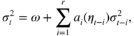
Autoregressive conditionally heteroscedastic (ARCH) models were introduced by Engle (1982), and their GARCH (generalised ARCH) extension is due to Bollerslev (1986). In these models, the key concept is the conditional variance, that is, the variance conditional on the past. In the classical GARCH models, the conditional variance is expressed as a linear function of the squared past values of the series. This particular specification is able to capture the main stylised facts characterising financial series, as described in Chapter 1. At the same time, it is simple enough to allow for a complete study of the solutions. The ‘linear’ structure of these models can be displayed through several representations that will be studied in this chapter.
We first present definitions and representations of GARCH models. Then we establish the strict and second‐order stationarity conditions. Starting with the first‐order GARCH model, for which the proofs are easier and the results are more explicit, we extend the study to the general case. We also study the so‐called ARCH(∞) models, which allow for a slower decay of squared‐return autocorrelations. Then, we consider the existence of moments and the properties of the autocorrelation structure. We conclude this chapter by examining forecasting issues.
2.1 Definitions and Representations
We start with a definition of GARCH processes based on the first two conditional moments.
Equation (2.1) can be written in a more compact way as
where
B
is the standard backshift operator (![]() and
and ![]() for any integer
i
), and
α
and
β
are polynomials of degrees
q
and
p
, respectively:
for any integer
i
), and
α
and
β
are polynomials of degrees
q
and
p
, respectively:

If β(z) = 0 we have

and the process is called an ARCH(
q
) process.
1
By definition, the innovation of the process ![]() is the variable
is the variable ![]() . Substituting in Eq. ( 2.1) the variables
. Substituting in Eq. ( 2.1) the variables ![]() by
by ![]() , we get the representation
, we get the representation

where
r = max(p, q), with the convention
α
i
= 0 (
β
j
= 0) if
i > q
(
j > p
). This equation has the linear structure of an ARMA model, allowing for simple computation of the linear predictions. Under additional assumptions (implying the second‐order stationarity of ![]() ), we can state that if (ε
t
) is GARCH(p, q), then
), we can state that if (ε
t
) is GARCH(p, q), then ![]() is an ARMA(r, p) process. In particular, the square of an ARCH(
q
) process admits, if it is stationary, an AR(
q
) representation. The ARMA representation will be useful for the estimation and identification of GARCH processes.
2
is an ARMA(r, p) process. In particular, the square of an ARCH(
q
) process admits, if it is stationary, an AR(
q
) representation. The ARMA representation will be useful for the estimation and identification of GARCH processes.
2
Definition 2.1 does not directly provide a solution process satisfying those conditions. The next definition is more restrictive but allows explicit solutions to be obtained. The link between the two definitions will be given in Remark 2.5. Let η denote a probability distribution with null expectation and unit variance.
GARCH processes in the sense of Definition 2.1 are sometimes called semi‐strong following the paper by Drost and Nijman (1993) on temporal aggregation. Substituting ε t − i by σ t − i η t − i in ( 2.1), we get

which can be written as follows:
where a i (z) = α i z 2 + β i , i = 1, …, r . This representation shows that the volatility process of a strong GARCH is the solution of an autoregressive equation with random coefficients.
Properties of Simulated Paths
Contrary to standard time series models (ARMA), the GARCH structure allows the magnitude of the noise ε
t
to be a function of its past values. Thus, periods with high‐volatility level (corresponding to large values of ![]() ) will be followed by periods where the fluctuations have a smaller amplitude. Figures 2.1–2.7 illustrate the volatility clustering for simulated GARCH models. Large absolute values are not uniformly distributed on the whole period, but tend to cluster. We will see that all these trajectories correspond to strictly stationary processes which, except for the ARCH(1) models of Figures 2.3–2.5, are also second‐order stationary. Even if the absolute values can be extremely large, these processes are not explosive, as can be seen from these figures. Higher values of
α
(theoretically,
α > 3.56 for the
) will be followed by periods where the fluctuations have a smaller amplitude. Figures 2.1–2.7 illustrate the volatility clustering for simulated GARCH models. Large absolute values are not uniformly distributed on the whole period, but tend to cluster. We will see that all these trajectories correspond to strictly stationary processes which, except for the ARCH(1) models of Figures 2.3–2.5, are also second‐order stationary. Even if the absolute values can be extremely large, these processes are not explosive, as can be seen from these figures. Higher values of
α
(theoretically,
α > 3.56 for the ![]() distribution, as will be established below) lead to explosive paths. Figures 2.6 and 2.7, corresponding to GARCH(1, 1) models, have been obtained with the same simulated sequence (η
t
). As we will see, permuting
α
and
β
does not modify the variance of the process but has an effect on the higher‐order moments. For instance the simulated process of Figure 2.7, with
α = 0.7 and
β = 0.2, does not admit a fourth‐order moment, in contrast to the process of Figure 2.6. This is reflected by the presence of larger absolute values in Figure 2.7. The two processes are also different in terms of persistence of shocks: when
β
approaches 1, a shock on the volatility has a persistent effect. On the other hand, when
α
is large, sudden volatility variations can be observed in response to shocks.
distribution, as will be established below) lead to explosive paths. Figures 2.6 and 2.7, corresponding to GARCH(1, 1) models, have been obtained with the same simulated sequence (η
t
). As we will see, permuting
α
and
β
does not modify the variance of the process but has an effect on the higher‐order moments. For instance the simulated process of Figure 2.7, with
α = 0.7 and
β = 0.2, does not admit a fourth‐order moment, in contrast to the process of Figure 2.6. This is reflected by the presence of larger absolute values in Figure 2.7. The two processes are also different in terms of persistence of shocks: when
β
approaches 1, a shock on the volatility has a persistent effect. On the other hand, when
α
is large, sudden volatility variations can be observed in response to shocks.

Figure 2.1
Simulation of size 500 of the ARCH(1) process with
ω = 1,
α = 0.5 and  .
.

Figure 2.2 Simulation of size 500 of the ARCH(1) process with
ω = 1,
α = 0.95 and 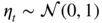 .
.

Figure 2.3
Simulation of size 500 of the ARCH(1) process with
ω = 1,
α = 1.1 and  .
.

Figure 2.4
Simulation of size 200 of the ARCH(1) process with
ω = 1,
α = 3 and  .
.

Figure 2.5 Observations 100–140 of Figure 2.4.

Figure 2.6
Simulation of size 500 of the GARCH(1, 1) process with
ω = 1,
α = 0.2,
β = 0.7 and  .
.

Figure 2.7
Simulation of size 500 of the GARCH(1, 1) process with
ω = 1,
α = 0.7,
β = 0.2 and  .
.
2.2 Stationarity Study
This section is concerned with the existence of stationary solutions (in the strict and second‐order senses) to model (2.5). We are mainly interested in non‐anticipative solutions, that is, processes (ε t ) such that ε t is a measurable function of the variables η t − s , s ≥ 0. For such processes, σ t is independent of the σ ‐field generated by {η t + h , h ≥ 0} and ε t is independent of the σ ‐field generated by {η t + h , h > 0}. It will be seen that such solutions are also ergodic. The concept of ergodicity is discussed in Appendix A.1. We first consider the GARCH(1, 1) model, which can be studied in a more explicit way than the general case. For x > 0, let log+ x = max(log x, 0).
2.2.1 The GARCH(1,1) Case
When p = q = 1, model ( 2.5) has the form

with ω > 0, α ≥ 0, β ≥ 0. Let a(z) = αz 2 + β .
The next result shows that non‐stationary GARCH processes are explosive.
Figure 2.8 shows the zones of strict and second‐order stationarity for the strong GARCH(1, 1) model when ![]() . Note that the distribution of
η
t
only matters for the strict stationarity. As noted above, the frontier of the strict stationarity zone corresponds to a random walk (for the process log(h
t
− ω)). A similar interpretation holds for the second‐order stationarity zone. If
α + β = 1 we have
. Note that the distribution of
η
t
only matters for the strict stationarity. As noted above, the frontier of the strict stationarity zone corresponds to a random walk (for the process log(h
t
− ω)). A similar interpretation holds for the second‐order stationarity zone. If
α + β = 1 we have

Figure 2.8
Stationarity regions for the GARCH(1, 1) model when  : 1, second‐order stationarity; 1 and 2, strict stationarity; 3, non‐stationarity.
Thus, since the last term in this equality is centred and uncorrelated with any variable belonging to the past of h t − 1 , the process (h t ) is a random walk. The corresponding GARCH process is called integrated GARCH (or IGARCH(1, 1)) and will be studied later: it is strictly stationary, has an infinite variance, and a conditional variance which is a random walk (with a positive drift).
2.2.2 The General Case
In the general case of a strong GARCH(p, q) process, the following vector representation will be useful. We have
where
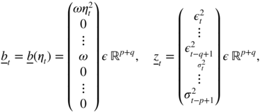
and

is a (p + q) × (p + q) matrix. In the ARCH(
q
) case, ![]() reduces to
reduces to ![]() and its
q − 1 first past values, and
A
t
to the upper‐left block of the above matrix. Equation (2.16) defines a first‐order vector autoregressive model, with positive and iid matrix coefficients. The distribution of
and its
q − 1 first past values, and
A
t
to the upper‐left block of the above matrix. Equation (2.16) defines a first‐order vector autoregressive model, with positive and iid matrix coefficients. The distribution of ![]() conditional on its infinite past coincides with its distribution conditional on
z
t − 1
only, which means that
conditional on its infinite past coincides with its distribution conditional on
z
t − 1
only, which means that ![]() is a Markov process. Model ( 2.16) is thus called the Markov representation of the GARCH(p, q) model. Iterating Eq. ( 2.16) yields
is a Markov process. Model ( 2.16) is thus called the Markov representation of the GARCH(p, q) model. Iterating Eq. ( 2.16) yields

provided that the series exists a.s.. Finding conditions ensuring the existence of this series is the object of what follows. Notice that the existence of the right‐hand vector in (2.18) does not ensure that its components are positive. One sufficient condition for
in the sense that all the components of this vector are strictly positive (but possibly infinite), is that
This condition is very simple to use but may not be necessary, as we will see in Section 2.3.2.
Strict Stationarity
The main tool for studying strict stationarity is the concept of the top Lyapunov exponent. Let A be a (p + q) × (p + q) matrix. The spectral radius of A , denoted by ρ(A), is defined as the greatest modulus of its eigenvalues. Let ‖ ⋅ ‖ denote any norm on the space of the (p + q) × (p + q) matrices. We have the following algebra result:
(Exercise 2.3). This property has the following extension to random matrices.
As for ARMA models, we are mostly interested in the non‐anticipative solutions (ε t ) to model ( 2.5), that is, those for which ε t belongs to the σ ‐field generated by {η t , η t − 1, …}.
We now give two illustrations allowing us to obtain more explicit stationarity conditions than in the theorem.
Figure 2.9, constructed from these simulations, gives a more precise idea of the strict stationarity region for an ARCH(2) process. We shall establish in Corollary 2.3 a result showing that any strictly stationary GARCH process admits small‐order moments. We begin with two lemmas which are of independent interest.

Figure 2.9 Stationarity regions for the ARCH(2) model: 1, second‐order stationarity; 1 and 2, strict stationarity; 3, non‐stationarity.
The following result, which is stated for any sequence of positive iid matrices, provides another characterisation of the strict stationarity of GARCH models.
Using Lemma 2.3 and Corollary 2.3 together, it can be seen that for s ∈ (0, 1],
The converse is generally true. For instance, we have for s ∈ (0, 1],
(Exercise 2.15).
Second‐Order Stationarity
The following theorem gives necessary and sufficient second‐order stationarity conditions.
IGARCH(p, q) Processes
When
the model is called an integrated GARCH(p, q) or IGARCH(p, q) model (see Engle and Bollerslev 1986). This name is justified by the existence of a unit root in the autoregressive part of representation ( 2.4) and is introduced by analogy with the integrated ARMA models, or ARIMA. However, this analogy can be misleading: there exists no (strict or second‐order) stationary solution of an ARIMA model, whereas an IGARCH model admits a strictly stationary solution under very general conditions. In the univariate case ( p = q = 1), the latter property is easily shown.
This property extends to the general case under slightly more restrictive conditions on the law of η t .
Note that this strictly stationary solution has an infinite variance in view of Theorem 2.5.
2.3 ARCH(∞)Representation *
A process (ε
t
) is called an ARCH(∞) process if there exists a sequence of iid variables (η
t
) such that
E(η
t
) = 0 and ![]() , and a sequence of constants
φ
i
≥ 0,
i = 1, …, and
φ
0 > 0 such that
, and a sequence of constants
φ
i
≥ 0,
i = 1, …, and
φ
0 > 0 such that
This class obviously contains the ARCH(q) process, and we shall see that it more generally contains the GARCH(p, q) process.
2.3.1 Existence Conditions
The existence of a stationary ARCH(∞) process requires assumptions on the sequences (φ i ) and (η t ). The following result gives an existence condition.
Equality ( 2.42) is called a Volterra expansion (see Priestley 1988). It shows in particular that, under the conditions of the theorem, if φ 0 = 0, the unique strictly stationary and non‐anticipative solution of the ARCH(∞) model is the identically null sequence. An application of Theorem 2.6, obtained for s = 1, is that the condition

ensures the existence of a second‐order stationary ARCH(∞) process. If
it can be shown (see Giraitis, Kokoszka, and Leipus 2000a) that ![]() ,
, ![]() for all
h
and
for all
h
and

The fact that the squares have positive autocovariances will be verified later in the GARCH case (see Section 2.5). In contrast to GARCH processes, for which they decrease at exponential rate, the autocovariances of the squares of ARCH(∞) can decrease at the rate h −γ with γ > 1 arbitrarily close to 1. A strictly stationary process of the form ( 2.40) such that

is called integrated ARCH(∞), or IARCH(∞). Notice that an IARCH(∞) process has infinite variance. Indeed, if ![]() , then, by ( 2.40),
σ
2 = φ
0 + σ
2
, which is impossible. From Theorem 2.8, the strictly stationary solutions of IGARCH models (see Corollary 2.5) admit IARCH(∞) representations. The next result provides a condition for the existence of IARCH(∞) processes.
, then, by ( 2.40),
σ
2 = φ
0 + σ
2
, which is impossible. From Theorem 2.8, the strictly stationary solutions of IGARCH models (see Corollary 2.5) admit IARCH(∞) representations. The next result provides a condition for the existence of IARCH(∞) processes.
Other integrated processes are the long‐memory ARCH, for which the rate of decrease of the φ i is not geometric.
2.3.2 ARCH(∞) Representation of a GARCH
It is sometimes useful to consider the ARCH(∞) representation of a GARCH(p, q) process. For instance, this representation allows the conditional variance ![]() of ε
t
to be written explicitly as a function of its infinite past. It also allows the positivity condition (2.20) on the coefficients to be weakened. Let us first consider the GARCH(1, 1) model. If
β < 1, we have
of ε
t
to be written explicitly as a function of its infinite past. It also allows the positivity condition (2.20) on the coefficients to be weakened. Let us first consider the GARCH(1, 1) model. If
β < 1, we have

In this case, we have

The condition A s μ 2s < 1 thus takes the form
For example, if α + β < 1 this condition is satisfied for s = 1. However, second‐order stationarity is not necessary for the validity of (2.46). Indeed, if (ε t ) denotes the strictly stationary and non‐anticipative solution of the GARCH(1, 1) model, then, for any q ≥ 1,

By Corollary 2.3 there exists
s ∈ (0, 1[ such that ![]() . It follows that
. It follows that ![]() So
So ![]() converges a.s. to 0 and, by letting
q
go to infinity in (2.47), we get ( 2.46). More generally, we have the following property.
converges a.s. to 0 and, by letting
q
go to infinity in (2.47), we get ( 2.46). More generally, we have the following property.
The ARCH(∞) representation can be used to weaken the condition ( 2.20) imposed to ensure the positivity of ![]() . Consider the GARCH(p, q) model with
ω > 0, without any a priori positivity constraint on the coefficients
α
i
and
β
j
, and assuming that the roots of the polynomial
ℬ(z) = 1 − β
1
z − ⋯ − β
p
z
p
have moduli strictly greater than 1. The coefficients
φ
i
introduced in ( 2.48) are then well defined, and under the assumption
. Consider the GARCH(p, q) model with
ω > 0, without any a priori positivity constraint on the coefficients
α
i
and
β
j
, and assuming that the roots of the polynomial
ℬ(z) = 1 − β
1
z − ⋯ − β
p
z
p
have moduli strictly greater than 1. The coefficients
φ
i
introduced in ( 2.48) are then well defined, and under the assumption
we have

Indeed,
φ
0 > 0 because otherwise
B(1) ≤ 0, which would imply the existence of a root inside the unit circle since
ℬ(0) = 1. Moreover, the proofs of the sufficient parts of Theorem 2.4, Lemma 2.3, and Corollary 2.3 do not use the positivity of the coefficients of the matrices
A
t
. It follows that if the top Lyapunov exponent of the sequence (A
t
) is such that
γ < 0, the variable ![]() is a.s. finite‐valued. To summarise, the conditions
is a.s. finite‐valued. To summarise, the conditions
imply that there exists a strictly stationary and non‐anticipative solution to model ( 2.5). The condition (2.49) is not generally simple to use, however, because it implies an infinity of constraints on the coefficients α i and β j . In the ARCH( q ) case, it reduces to the condition ( 2.20), that is, α i ≥ 0, i = 1, …, q . Similarly, in the GARCH(1, 1) case, it is necessary to have α 1 ≥ 0 and β 1 ≥ 0. However, for p ≥ 1 and q > 1, the condition ( 2.20) can be weakened (Exercise 2.16).
2.3.3 Long‐Memory ARCH
The introduction of long memory into the volatility can be motivated by the observation that the empirical autocorrelations of the squares, or of the absolute values, of financial series decay very slowly in general (see for example Table 2.1). We shall see that it is possible to reproduce this property by introducing ARCH(∞) processes, with a sufficiently slow decay of the modulus of the coefficients φ i . 8 A process (X t ) is said to have long memory if it is second‐order stationary and satisfies, for h → ∞,
and
K
is a non‐zero constant. An alternative definition relies on distinguishing ‘intermediate‐memory’ processes for which
d < 0 and thus ![]() , and ‘long‐memory’ processes for which
d ∈ (0, 1/2[ and thus
, and ‘long‐memory’ processes for which
d ∈ (0, 1/2[ and thus ![]() (see Brockwell and Davis 1991, p. 520). The autocorrelations of an ARMA process decrease at exponential rate when the lag increases. The need for processes with a slower autocovariance decay leads to the introduction of the fractionary ARIMA models. These models are defined through the fractionary difference operator
(see Brockwell and Davis 1991, p. 520). The autocorrelations of an ARMA process decrease at exponential rate when the lag increases. The need for processes with a slower autocovariance decay leads to the introduction of the fractionary ARIMA models. These models are defined through the fractionary difference operator

Denoting by π j the coefficient of B j in this sum, it can be shown that π j ∼Kj −d − 1 when j → ∞, where K is a constant depending on d . An ARIMA(p, d, q) process with d ∈ ( − 0.5, 0.5) is defined as a stationary solution of
where ε t is a white noise, and ψ and θ are polynomials of degrees p and q , respectively. If the roots of these polynomials are all outside the unit disk, the unique stationary and purely deterministic solution is causal, invertible and its covariances satisfy condition (2.50) (see Brockwell and Davis 1991, Theorem 13.2.2.). By analogy with the ARIMA models, the class of FIGARCH(p, d, q) processes is defined by the equations

where ψ and θ are polynomials of degrees p and q , respectively, such that ψ(0) = θ(0) = 1, the roots of ψ have moduli strictly greater than 1 and φ i ≥ 0, where the φ i are defined by

We have
φ
i
∼Ki
−d − 1
, where
K
is a positive constant, when
i → ∞ and ![]() . The process introduced in (2.51) is thus IARCH(∞), provided it exists. Note that existence of this process cannot be obtained by Theorem 2.7 because, for the FIGARCH model, the
φ
i
decrease more slowly than the geometric rate. The following result, which is a consequence of Theorem 2.6, and whose proof is the subject of Exercise 2.22, provides another sufficient condition for the existence of IARCH(∞) processes.
. The process introduced in (2.51) is thus IARCH(∞), provided it exists. Note that existence of this process cannot be obtained by Theorem 2.7 because, for the FIGARCH model, the
φ
i
decrease more slowly than the geometric rate. The following result, which is a consequence of Theorem 2.6, and whose proof is the subject of Exercise 2.22, provides another sufficient condition for the existence of IARCH(∞) processes.
This result can be used to prove the existence of FIGARCH(p,d,q) processes for d ∈ (0,1) sufficiently close to 1, if the distribution of ![]() is assumed to be non‐degenerate (hence,
is assumed to be non‐degenerate (hence, ![]() ); see Douc, Roueff, and Soulier (2008). The FIGARCH process of Corollary 2.6 does not admit a finite second‐order moment. Its square is thus not a long‐memory process in the sense of definition ( 2.50). More generally, it can be shown that the squares of a ARCH(∞) processes do not have the long‐memory property. This motivated the introduction of an alternative class, called linear ARCH (LARCH) and defined by
); see Douc, Roueff, and Soulier (2008). The FIGARCH process of Corollary 2.6 does not admit a finite second‐order moment. Its square is thus not a long‐memory process in the sense of definition ( 2.50). More generally, it can be shown that the squares of a ARCH(∞) processes do not have the long‐memory property. This motivated the introduction of an alternative class, called linear ARCH (LARCH) and defined by

Under appropriate conditions, this model is compatible with the long‐memory property for ![]() .
.
2.4 Properties of the Marginal Distribution
We have seen that, under quite simple conditions, a GARCH(p, q) model admits a strictly stationary solution (ε t ). However, the marginal distribution of the process (ε t ) is never known explicitly. The aim of this section is to highlight some properties of this distribution through the marginal moments.
2.4.1 Even‐Order Moments
We are interested in finding existence conditions for the moments of order 2m , where m is any positive integer. 9 Let ⊗ denote the tensor product, or Kronecker product, and recall that it is defined as follows: for any matrices A = (a ij ) and B , we have A ⊗ B = (a ij B). For any matrix A , let A ⊗m = A ⊗ ⋯ ⊗ A . We have the following result.
This example shows that for a non‐trivial GARCH process, that is, when the α i and β j are not all equal to zero, the moments cannot exist for any order.
2.4.2 Kurtosis
An easy way to measure the size of distribution tails is to use the kurtosis coefficient. This coefficient is defined, for a centred (zero‐mean) distribution, as the ratio of the fourth‐order moment, which is assumed to exist, to the squared second‐order moment. This coefficient is equal to 3 for a normal distribution, this value serving as a gauge for the other distributions. In the case of GARCH processes, it is interesting to note the difference between the tails of the marginal and conditional distributions. For a strictly stationary solution, (ε
t
) of the GARCH(p, q) model defined by ( 2.5), the conditional moments of order
k
are proportional to ![]() :
:
The kurtosis coefficient of this conditional distribution is thus constant and equal to the kurtosis coefficient of η t . For a general process of the form
where σ t is a measurable function of the past of ε t , η t is independent of this past and (η t ) is iid centred, the kurtosis coefficient of the stationary marginal distribution is equal, provided that it exists, to

where ![]() denotes the kurtosis coefficient of (η
t
). It can thus be seen that the tails of the marginal distribution of (ε
t
) are fatter when the variance of
denotes the kurtosis coefficient of (η
t
). It can thus be seen that the tails of the marginal distribution of (ε
t
) are fatter when the variance of ![]() is large relative to the squared expectation. The minimum (corresponding to the absence of ARCH effects) is given by the kurtosis coefficient of (η
t
),
is large relative to the squared expectation. The minimum (corresponding to the absence of ARCH effects) is given by the kurtosis coefficient of (η
t
),
with equality if and only if ![]() is a.s. constant. In the GARCH(1, 1) case we thus have, from the previous calculations,
is a.s. constant. In the GARCH(1, 1) case we thus have, from the previous calculations,

The excess kurtosis coefficients of ε t and η t , relative to the normal distribution, are related by

The excess kurtosis of ε t increases with that of η t and when the GARCH coefficients approach the zone of non‐existence of the fourth‐order moment. Notice the asymmetry between the GARCH coefficients in the excess kurtosis formula. For the general GARCH(p, q), we have the following result.
It will be seen in Chapter 7 that the Gaussian quasi‐maximum likelihood estimator of the coefficients of a GARCH model is consistent and asymptotically normal even if the distribution of the variables η t is not Gaussian. Since the autocorrelation function of the squares of the GARCH process does not depend on the law of η t , the autocorrelations obtained by replacing the unknown coefficients by their estimates are generally very close to the empirical autocorrelations. In contrast, the kurtosis coefficients obtained from the theoretical formula, by replacing the coefficients by their estimates and the kurtosis of η t by 3, can be very far from the coefficients obtained empirically. This is not very surprising since the preceding result shows that the difference between the kurtosis coefficients of ε t computed with a Gaussian and a non‐Gaussian distribution for η t ,

is not bounded as
a
approaches ![]() .
.
2.5 Autocovariances of the Squares of a GARCH
We have seen that if (ε
t
) is a GARCH process which is fourth‐order stationary, then ![]() is an ARMA process. It must be noted that this ARMA is very constrained, as can be seen from representation ( 2.4): the order of the AR part is larger than that of the MA part, and the AR coefficients are greater than those of the MA part, which are positive. We shall start by examining some consequences of these constraints on the autocovariances of
is an ARMA process. It must be noted that this ARMA is very constrained, as can be seen from representation ( 2.4): the order of the AR part is larger than that of the MA part, and the AR coefficients are greater than those of the MA part, which are positive. We shall start by examining some consequences of these constraints on the autocovariances of ![]() . Then we shall show how to compute these autocovariances explicitly.
. Then we shall show how to compute these autocovariances explicitly.
2.5.1 Positivity of the Autocovariances
For a GARCH(1, 1) model such that ![]() , the autocorrelations of the squares take the form
, the autocorrelations of the squares take the form
where

(Exercise 2.8). It follows immediately that these autocorrelations are non‐negative. The next property generalises this result.
Note that the property of positive autocorrelations for the squares, or for the absolute values, is typically observed on real financial series (see, for instance, the second row of Table 2.1).
2.5.2 The Autocovariances Do Not Always Decrease
Formulas (2.61) and (2.62) show that for a GARCH(1,1) process, the autocorrelations of the squares decrease. An illustration is provided in Figure 2.11. A natural question is whether this property remains true for more general GARCH(p, q) processes. The following computation shows that this is not the case. Consider an ARCH(2) process admitting moments of order 4 (the existence condition and the computation of the fourth‐order moment are the subject of Exercise 2.8):

Figure 2.11
Autocorrelation function (a) and partial autocorrelation function (b) of the squares of the GARCH(1, 1) model ε
t
= σ
t
η
t
,  , (η
t
) iid 풩(0, 1).
, (η
t
) iid 풩(0, 1).
We know that ![]() is an AR(2) process, whose autocorrelation function satisfies
is an AR(2) process, whose autocorrelation function satisfies
It readily follows that

and hence that
The latter equality is, of course, true for the ARCH(1) process ( α 2 = 0) but is not true for any (α 1, α 2). Figure 2.12 gives an illustration of this non‐decreasing feature of the first autocorrelations (and partial autocorrelations). The sequence of autocorrelations is, however, decreasing after a certain lag (Exercise 2.18).

Figure 2.2
Autocorrelation function (a) and partial autocorrelation function (b) of the squares of the ARCH(2) process ε
t
= σ
t
η
t
,  , (η
t
) iid 풩(0, 1).
, (η
t
) iid 풩(0, 1).
2.5.3 Explicit Computation of the Autocovariances of the Squares
The autocorrelation function of ![]() will play an important role in identifying the orders of the model. This function is easily obtained from the ARMA(max(p, q), p) representation
will play an important role in identifying the orders of the model. This function is easily obtained from the ARMA(max(p, q), p) representation

The autocovariance function is more difficult to obtain (Exercise 2.9) because one has to compute
One can use the method of Section 2.4.1. Consider the vector representation
defined in ( 2.16) and ( 2.17). Using the independence between ![]() and
and ![]() , together with elementary properties of the Kronecker product ⊗, we get
, together with elementary properties of the Kronecker product ⊗, we get
Thus
where
To compute
A
(m)
, we can use the decomposition ![]() , where
B
and
C
are deterministic matrices. We then have, letting
, where
B
and
C
are deterministic matrices. We then have, letting ![]() ,
,
We obtain ![]() and
and ![]() similarly. All the components of
similarly. All the components of ![]() are equal to
ω/(1 − ∑ α
i
− ∑ β
i
). Note that for
h > 0, we have
are equal to
ω/(1 − ∑ α
i
− ∑ β
i
). Note that for
h > 0, we have

Let ![]() . The following algorithm can be used:
. The following algorithm can be used:
- Define the vectors
 ,
,  ,
,  , and the matrices
  ,
,  ,
A
(1)
,
A
(2)
as a function of
α
i
,
β
i
, and
ω
,
μ
4
.
,
A
(1)
,
A
(2)
as a function of
α
i
,
β
i
, and
ω
,
μ
4
. - Compute
 from Eq. (2.63).
 - For
h = 1, 2, …, compute
 from Eq. (2.64).
 - For
h = 0, 1, …, compute
 .
.
This algorithm is not very efficient in terms of computation time and memory space, but it is easy to implement.
2.6 Theoretical Predictions
The definition of GARCH processes in terms of conditional expectations allows us to compute the optimal predictions of the process and its square given its infinite past. Let (ε t ) be a stationary GARCH(p, q) process, in the sense of Definition 2.1. The optimal prediction (in the L 2 sense) of ε t given its infinite past is 0 by Definition 2.1(i). More generally, for h + 1 > 0,
which shows that the optimal prediction of any future variable given the infinite past is zero. The main attraction of GARCH models obviously lies not in the prediction of the GARCH process itself but in the prediction of its square. The optimal prediction of ![]() given the infinite past of ε
t
is
given the infinite past of ε
t
is ![]() . More generally, the predictions at horizon
h ≥ 0 are obtained recursively by
. More generally, the predictions at horizon
h ≥ 0 are obtained recursively by

with, for i ≤ h ,
for i > h ,
and for i ≥ h ,
These predictions coincide with the optimal linear predictions of the future values of ![]() given its infinite past. Note that there exists a more general class of GARCH models (weak GARCH) for which the two types of predictions, optimal and linear optimal, do not necessarily coincide. Weak GARCH representations appear, in particular, when GARCH are temporally aggregated (see Drost and Werker, 1996; Drost, Nijman and Werker 1998), when they are observed with a measurement error as in Gouriéroux, Monfort and Renault (1993) andKing, Sentana and Wadhwani (1994), or for the beta‐ARCHof Diebolt and Guégan (1991). See Francq and Zakoïan (2000) for other examples.
given its infinite past. Note that there exists a more general class of GARCH models (weak GARCH) for which the two types of predictions, optimal and linear optimal, do not necessarily coincide. Weak GARCH representations appear, in particular, when GARCH are temporally aggregated (see Drost and Werker, 1996; Drost, Nijman and Werker 1998), when they are observed with a measurement error as in Gouriéroux, Monfort and Renault (1993) andKing, Sentana and Wadhwani (1994), or for the beta‐ARCHof Diebolt and Guégan (1991). See Francq and Zakoïan (2000) for other examples.
It is important to note that ![]() is the conditional variance of the prediction error of ε
t + h
. Hence, the accuracy of the predictions depends on the past: it is particularly low after a turbulent period, that is, when the past values are large in absolute value (assuming that the coefficients
α
i
and
β
j
are non‐negative). This property constitutes a crucial difference with standard ARMA models, for which the magnitude of the prediction intervals is constant, for a given horizon.
is the conditional variance of the prediction error of ε
t + h
. Hence, the accuracy of the predictions depends on the past: it is particularly low after a turbulent period, that is, when the past values are large in absolute value (assuming that the coefficients
α
i
and
β
j
are non‐negative). This property constitutes a crucial difference with standard ARMA models, for which the magnitude of the prediction intervals is constant, for a given horizon.
Figures 2.13–2.16, based on simulations, allow us to visualise this difference. In Figure 2.13, obtained from a Gaussian white noise, the predictions at horizon 1 have a constant variance: the confidence interval [−1.96, 1.96] contains roughly 95% of the realisations. Using a constant interval for the next three series, displayed in Figures 2.14–2.16, would imply very bad results. In contrast, the intervals constructed here (for conditionally Gaussian distributions, with zero mean and variance ![]() ) do contain about 95% of the observations: in the quiet periods a small interval is enough, whereas in turbulent periods, the variability increases and larger intervals are needed.
) do contain about 95% of the observations: in the quiet periods a small interval is enough, whereas in turbulent periods, the variability increases and larger intervals are needed.
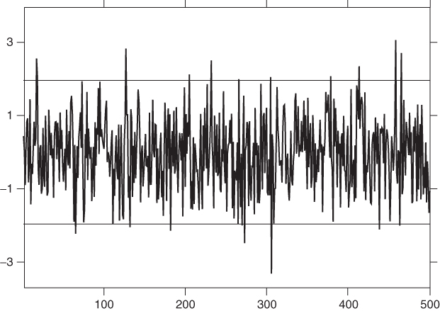
Figure 2.3 Prediction intervals at horizon 1, at 95%, for the strong 풩(0, 1) white noise.

Figure 2.4 Prediction intervals at horizon 1, at 95%, for the GARCH(1, 1) process simulated with ω = 1, α = 0.1, β = 0.8 and 풩(0, 1) distribution for (η t ).

Figure 2.15 Prediction intervals at horizon 1, at 95%, for the GARCH(1, 1) process simulated with ω = 1, α = 0.6, β = 0.2 and 풩(0, 1) distribution for (η t ).

Figure 2.6 Prediction intervals at horizon 1, at 95%, for the GARCH(1, 1) process simulated with ω = 1, α = 0.7, β = 0.3 and 풩(0, 1) distribution for (η t ).
For a strong GARCH process it is possible to go further, by computing optimal predictions of the powers of ![]() , provided that the corresponding moments exist for the process (η
t
). For instance, computing the predictions of
, provided that the corresponding moments exist for the process (η
t
). For instance, computing the predictions of ![]() allows us to evaluate the variance of the prediction errors of
allows us to evaluate the variance of the prediction errors of ![]() . However, these computations are tedious, the linearity property being lost for such powers.
. However, these computations are tedious, the linearity property being lost for such powers.
When the GARCH process is not directly observed but is the innovation of an ARMA process, the accuracy of the prediction at some date t directly depends of the magnitude of the conditional heteroscedasticity at this date. Consider, for instance, a stationary AR(1) process, whose innovation is a GARCH(1, 1) process:

where ω > 0, α ≥ 0, β ≥ 0, α + β ≤ 1 and ∣φ ∣ < 1. We have, for h ≥ 0,
Hence,
since the past of X t coincides with that of its innovation ε t . Moreover,

Since ![]() and, for
i ≥ 1,
and, for
i ≥ 1,

we have
Consequently,

if φ 2 ≠ α + β and

if
φ
2 = α + β
. The coefficient of ![]() always being positive, it can be seen that the variance of the prediction at horizon
h
increases linearly with the difference between the conditional variance at time
t
and the unconditional variance of ε
t
. A large negative difference (corresponding to a low‐volatility period) thus results in highly accurate predictions. Conversely, the accuracy deteriorates when
always being positive, it can be seen that the variance of the prediction at horizon
h
increases linearly with the difference between the conditional variance at time
t
and the unconditional variance of ε
t
. A large negative difference (corresponding to a low‐volatility period) thus results in highly accurate predictions. Conversely, the accuracy deteriorates when ![]() is large. When the horizon
h
increases, the importance of this factor decreases. If
h
tends to infinity, we retrieve the unconditional variance of
X
t
:
is large. When the horizon
h
increases, the importance of this factor decreases. If
h
tends to infinity, we retrieve the unconditional variance of
X
t
:
Now we consider two non‐stationary situations. If ∣φ ∣ = 1, and initialising, for instance at 0, all the variables at negative dates (because here the infinite pasts of X t and ε t do not coincide), the previous formula becomes

Thus, the impact of the observations before time t does not vanish as h increases. It becomes negligible, however, compared to the deterministic part which is proportional to h . If α + β = 1 (IGARCH(1, 1) errors), we have
and it can be seen that the impact of the past variables on the variance of the predictions remains constant as the horizon increases. This phenomenon is called persistence of shocks on the volatility. Note, however, that, as in the preceding case, the non‐random part of the decomposition of Var(ε t + i ∣ ε u , u < t) becomes dominant when the horizon tends to infinity. The asymptotic precision of the predictions of ε t is null, and this is also the case for X t since
2.7 Bibliographical Notes
The strict stationarity of the GARCH(1, 1) model was first studied by Nelson (1990a) under the assumption ![]() . His results were extended by Klüppelberg, Lindner, and Maller (2004) to the case of
. His results were extended by Klüppelberg, Lindner, and Maller (2004) to the case of ![]() . For GARCH(p, q) models, the strict stationarity conditions were established by Bougerol and Picard (1992b). For model ( 2.16), where
. For GARCH(p, q) models, the strict stationarity conditions were established by Bougerol and Picard (1992b). For model ( 2.16), where ![]() is a strictly stationary and ergodic sequence with a logarithmic moment, Brandt (1986) showed that
γ < 0 ensures the existence of a unique strictly stationary solution. In the case where
is a strictly stationary and ergodic sequence with a logarithmic moment, Brandt (1986) showed that
γ < 0 ensures the existence of a unique strictly stationary solution. In the case where ![]() is iid, Bougerol and Picard (1992a) established the converse property showing that, under an irreducibility condition, a necessary condition for the existence of a strictly stationary and non‐anticipative solution is that
γ < 0. Liu (2006) used representation ( 2.30) to obtain stationarity conditions for more general GARCH models. The second‐order stationarity condition for the GARCH(p, q) model was obtained by Bollerslev (1986), as well as the existence of an ARMA representation for the square of a GARCH (see also Bollerslev 1988). Nelson and Cao (1992) obtained necessary and sufficient positivity conditions for the GARCH(p, q) model. These results were extended by Tsai and Chan (2008). The ‘zero‐drift’ GARCH(1,1) model in which ω = 0 was studied by Hafner and Preminger (2015) and Li et al. (2017). In the latter article it was shown that, though non‐stationary, the zero‐drift GARCH(1, 1) model is stable when γ = 0, with its sample paths oscillating randomly between zero and infinity over time.
is iid, Bougerol and Picard (1992a) established the converse property showing that, under an irreducibility condition, a necessary condition for the existence of a strictly stationary and non‐anticipative solution is that
γ < 0. Liu (2006) used representation ( 2.30) to obtain stationarity conditions for more general GARCH models. The second‐order stationarity condition for the GARCH(p, q) model was obtained by Bollerslev (1986), as well as the existence of an ARMA representation for the square of a GARCH (see also Bollerslev 1988). Nelson and Cao (1992) obtained necessary and sufficient positivity conditions for the GARCH(p, q) model. These results were extended by Tsai and Chan (2008). The ‘zero‐drift’ GARCH(1,1) model in which ω = 0 was studied by Hafner and Preminger (2015) and Li et al. (2017). In the latter article it was shown that, though non‐stationary, the zero‐drift GARCH(1, 1) model is stable when γ = 0, with its sample paths oscillating randomly between zero and infinity over time.
GARCH are not the only models that generate uncorrelated times series with correlated squares. Another class of interest which shares these characteristics is that of the all‐pass time series models (ARMA models in which the roots of the AR polynomials are reciprocals of roots of the MA polynomial and vice versa) studied by Breidt, Davis, and Trindade (2001).
ARCH(∞) models were introduced by Robinson (1991); see Giraitis, Leipus, and Surgailis (2009) for the study of these models. The condition for the existence of a strictly stationary ARCH(∞) process was established by Robinson and Zaffaroni (2006) and Douc, Roueff, and Soulier (2008). The condition for the existence of a second‐order stationary solution, as well as the positivity of the autocovariances of the squares, were obtained by Giraitis, Kokoszka, and Leipus (2000a). Theorems 2.8 and 2.7 were proven by Kazakevičius and Leipus (2002, 2003). The uniqueness of an ARCH(∞) solution is discussed in Kazakevičius and Leipus (2007). The asymptotic properties of quasi‐maximum likelihood estimators (see Chapter 7) were established by Robinson and Zaffaroni (2006). See Doukhan, Teyssière, and Winant (2006) for the study of multivariate extensions of ARCH(∞) models. The introduction of FIGARCH models is due to Baillie, Bollerslev, and Mikkelsen (1996), but the existence of solutions was recently established by Douc, Roueff, and Soulier (2008), where Corollary 2.6 is proven. LARCH(∞) models were introduced by Robinson (1991) and their probability properties studied by Giraitis, Robinson, and Surgailis (2000b), Giraitis and Surgailis (2002), Berkes and Horváth (2003a), and Giraitis et al. (2004). The estimation of such models has been studied by Beran and Schützner (2009), Truquet (2008), and Francq and Zakoïan (2009c).
The fourth‐order moment structure and the autocovariances of the squares of GARCH processes were analysed by Milhøj (1984), Karanasos (1999), and He and Teräsvirta (1999). The necessary and sufficient condition for the existence of even‐order moments was established by Ling and McAleer (2002a), the sufficient part having been obtained by Chen and An 1998. Ling and McAleer (2002b) derived an existence condition for the moment of order s , with s > 0, for a family of GARCH processes including the standard model and the extensions presented in Chapter 4. The computation of the kurtosis coefficient for a general GARCH(p, q) model is due to Bai, Russell, and Tiao (2004).
Several authors have studied the tail properties of the stationary distribution. See Mikosch and Stărică (2000), Borkovec and Klüppelberg (2001), Basrak, Davis, and Mikosch (2002), and Davis and Mikosch (2009a,b). See Embrechts, Klüppelberg and Mikosch (1997) for a classical reference on extremal events.
Andersen and Bollerslev (1998) discussed the predictive qualities of GARCH, making a clear distinction between the prediction of volatility and that of the squared returns (Exercise 2.23).
2.8 Exercises
2.1 (Non‐correlation of ε t with any function of its past?)
For a GARCH process does Cov(ε t , f(ε t − h )) = 0 hold for any function f and any h > 0?
- 2.2 (Strict stationarity of GARCH(1, 1) for two laws of ηt) For the GARCH(1, 1) give an explicit strict stationarity condition in the two following cases: (i) the only possible values of η t are −1 and 1; (ii) η t follows a uniform distribution.
- 2.3 (Lyapunov coefficient of a constant sequence of matrices) Prove equality ( 2.21) for a diagonalisable matrix. Use the Jordan representation to extend this result to any square matrix.
- 2.4 (Lyapunov coefficient of a sequence of matrices) Consider the sequence (A t ) defined by A t = z t A , where (z t ) is an ergodic sequence of real random variables such that E log+ ∣ z t ∣ < ∞, and A is a square non‐random matrix. Find the Lyapunov coefficient γ of the sequence (A t ) and give an explicit expression for the condition γ < 0.
-
2.5 (Alternative definition of the top Lyapunov exponent)
- Show that, everywhere in Theorem 2.3, the matrix product A t A t−1…A 1 can be replaced by A −1 A −2…A −t .
- Justify the first convergence after (2.25).
- 2.6 (Multiplicative norms) Show the results of footnote 6 on page 28.
-
2.7 (Another vector representation of the GARCH(p, q) model) Verify that the vector
 allows us to define, for
p ≥ 1 and
q ≥ 2, a vector representation which is equivalent to those used in this chapter, of the form
allows us to define, for
p ≥ 1 and
q ≥ 2, a vector representation which is equivalent to those used in this chapter, of the form  .
. -
2.8 (Fourth‐order moment of an ARCH(2) process) Show that for an ARCH(2) model, the condition for the existence of the moment of order 4, with
 , is written as
Compute this moment.
-
2.9 (Direct computation of the autocorrelations and autocovariances of the square of a GARCH(1, 1) process) Find the autocorrelation and autocovariance functions of
 when (ε
t
) is solution of the GARCH(1, 1) model
when (ε
t
) is solution of the GARCH(1, 1) model
where
 and 1 − 3α
2 − β
2 − 2αβ > 0.
and 1 − 3α
2 − β
2 − 2αβ > 0. -
2.10 (Computation of the autocovariance of the square of a GARCH(1,1) process by the general method) Use the method of Section 2.5.3 to find the autocovariance function of
 when (ε
t
) is solution of a GARCH(1,1) model. Compare with the method used in Exercise 2.9.
when (ε
t
) is solution of a GARCH(1,1) model. Compare with the method used in Exercise 2.9. - 2.11 (Fekete's lemma for sub‐additive sequences) A sequence (a n ) n≥1 is called sub‐additive if a n+m ≤ a n + a m for all n and m. Show that we then have lim n‐>∞ a n /n = inf n≥1 a n /n.
-
2.12 (Characteristic polynomial of EAt) Let
A = EA
t
, where {A
t
, t ∈ ℤ} is the sequence defined in Eq. ( 2.17).
- Prove equality ( 2.38).
- If
 , show that
ρ(A) = 1.
, show that
ρ(A) = 1.
-
2.13 (A condition for a sequence Xn to be o(n)) Let (X
n
) be a sequence of identically distributed random variables, admitting a finite expectation. Show that

with probability 1. Prove that the convergence may fail if the expectation of X n does not exist (an iid sequence with density f(x) = x −2
 x ≥ 1
may be considered).
x ≥ 1
may be considered). - 2.14 (Expectation of a product of dependent random variables equal to the product of their expectations) Prove equality (2.31).
-
2.15 (Necessary condition for the existence of the moment of order 2s) Suppose that (ε
t
) is the strictly stationary solution of model ( 2.5) with
 for
s ∈ (0, 1]. Let2.66
for
s ∈ (0, 1]. Let2.66
- Show that when K → ∞,

- Use this result to prove that
 as
k → ∞ .
as
k → ∞ .
- Let (X
n
) a sequence of ℓ × m
matrices and
Y = (Y
1, …, Y
m
)′
a vector which is independent of (X
n
) and such that for all
i
, 0 < E|Y
i
|
s
< ∞. Show that, when
n → ∞,

- Let
A = EA
t
,
 and suppose there exists an integer
N
such that
and suppose there exists an integer
N
such that  (in the sense that all elements of this vector are strictly positive). Show that there exists
k
0 ≥ 1 such that
(in the sense that all elements of this vector are strictly positive). Show that there exists
k
0 ≥ 1 such that
- Deduce condition (2.35) from the preceding question.
- Is the condition α 1 + β 1 > 0 necessary?
- Show that when K → ∞,
- 2.16 (Positivity conditions) In the GARCH(1, q) case give a more explicit form for the conditions in ( 2.49). Show, by taking q = 2, that these conditions are less restrictive than ( 2.20).
-
2.17 (A minoration for the first autocorrelations of the square of an ARCH) Let (ε
t
) be an ARCH(
q
) process admitting moments of order 4. Show that, for
i = 1, …, q
,

- 2.18 (Asymptotic decrease of the autocorrelations of the square of an ARCH(2) process) Figure 2.12 shows that the first autocorrelations of the square of an ARCH(2) process, admitting moments of order 4, can be non‐decreasing. Show that this sequence decreases after a certain lag.
-
2.19 (Convergence in probability to −∞) If (X
n
) and (Y
n
) are two independent sequences of random variables such that
X
n
+ Y
n
→ − ∞ and
 in probability, then
Y
n
→ − ∞ in probability.
in probability, then
Y
n
→ − ∞ in probability. -
2.20 (GARCH model with a random coefficient) Proceeding as in the proof of Theorem 2.1, study the stationarity of the GARCH(1, 1) model with random coefficient
ω = ω(η
t − 1),2.67

under the usual assumptions and ω(η t − 1) > 0 a.s. Use the result of Exercise 2.19 to deal with the case γ ≔ E log a(η t ) = 0.
-
2.21 (RiskMetrics model) The RiskMetrics model used to compute the value at risk (see Chapter 11) relies on the following equations:

where 0 < λ < 1. Show that this model has no stationary and non trivial solution.
-
2.22 (IARCH(∞) models: proof of Corollary 2.6)
- In model ( 2.40), under the assumption
A
1 = 1, show that

- Suppose that condition ( 2.41) holds. Show that the function f : [p,1] ↦ ℝ defined by f(q) = log(A q μ 2q ) is convex. Compute its derivative at 1 and deduce that condition (2.52) holds.
- Establish the reciprocal and show that E|ε t | q < ∞ for any q ∈ [0, 2).
- In model ( 2.40), under the assumption
A
1 = 1, show that
-
2.23 (On the predictive power of GARCH) In order to evaluate the quality of the prediction of
 obtained by using the volatility of a GARCH(1, 1) model, econometricians have considered the linear regression
where
 is replaced by the volatility estimated from the model. They generally obtained a very small determination coefficient, meaning that the quality of the regression was bad. It this surprising? In order to answer that question compute, under the assumption that
  exists, the theoretical
R
2
defined by
exists, the theoretical
R
2
defined by
Show, in particular, that R 2 < 1/κ η .