
Appendix C
Helpful Formulas
C.1 Positive and Negative Parts
For any number ![]() , we define the positive part and negative part of x as, respectively:
, we define the positive part and negative part of x as, respectively:
(Some authors use ![]() .)
.)
The following identities hold:
For any ![]() , we have:
, we have:
If ![]() , then
, then
C.2 Standard Normal Random Variables
Let ![]() with pdf f and cdf F. Let
with pdf f and cdf F. Let ![]() and
and ![]() be the pdf and cdf, respectively, of the standard normal distribution.
be the pdf and cdf, respectively, of the standard normal distribution.
We define
for ![]() . Moreover,
. Moreover,
C.3 Loss Functions
Throughout, we use ![]() and
and ![]() to refer to the first‐ and second‐order loss functions, and
to refer to the first‐ and second‐order loss functions, and ![]() and
and ![]() to refer to the corresponding complementary loss functions.
1
It would be equally appropriate to use
to refer to the corresponding complementary loss functions.
1
It would be equally appropriate to use ![]() for the first‐order loss function, but we drop the superscript for notational simplicity, and often omit the phrase “first‐order” when describing this function and its complement. For the standard normal distribution, we replace n with
for the first‐order loss function, but we drop the superscript for notational simplicity, and often omit the phrase “first‐order” when describing this function and its complement. For the standard normal distribution, we replace n with ![]() in these functions.
in these functions.
C.3.1 General Continuous Distributions
Let X be a continuous random variable with pdf f and cdf F. Let ![]() be the complementary cdf. The loss function and complementary loss function are given by
be the complementary cdf. The loss function and complementary loss function are given by
The loss function and its complement are related as follows:
The derivatives of the loss function and its complement are given by
The loss function and its complement are therefore both convex.
The second‐order loss function and its complement are given by
The second‐order loss function and its complement are related as follows:
The derivatives of the second‐order loss function and its complement are given by
C.3.2 Standard Normal Distribution
Let ![]() , with pdf
, with pdf ![]() , cdf
, cdf ![]() , and complementary cdf
, and complementary cdf ![]() . The standard normal loss function, its complement, and their derivatives are given by
. The standard normal loss function, its complement, and their derivatives are given by
Also:
(The second equality follows from the fact that ![]() .)
.)
The second‐order standard normal loss function, its complement, and their derivatives are given by


C.3.3 Nonstandard Normal Distributions
Let ![]() with pdf f, cdf F, and complementary cdf
with pdf f, cdf F, and complementary cdf ![]() . The normal loss function can be computed using the standard normal loss function as follows:
. The normal loss function can be computed using the standard normal loss function as follows:
where ![]() . (In many instances, we assume
. (In many instances, we assume ![]() so that the probability that
so that the probability that ![]() is small; in these cases, we often replace the lower limit of the integral in (C.32) with 0.) The derivatives of
is small; in these cases, we often replace the lower limit of the integral in (C.32) with 0.) The derivatives of ![]() and
and ![]() are given by (C.15)–(C.16).
are given by (C.15)–(C.16).
The second‐order normal loss function and its complement are given by
C.3.4 General Discrete Distributions
Let X be a discrete random variable with pmf f and cdf F. Let ![]() be the complementary cdf. The loss function and complementary loss function are given by
be the complementary cdf. The loss function and complementary loss function are given by

The loss function and its complement are related as follows:
The second‐order loss function and its complement are given by


The second‐order loss function and its complement are related as follows:
If X is nonnegative, then equations C.37) and (C.40) can facilitate the calculation of ![]() and
and ![]() , since
, since ![]() and
and ![]() contain infinite sums, but
contain infinite sums, but ![]() and
and ![]() contain finite ones.
contain finite ones.
C.3.5 Poisson Distribution
Let ![]() with pmf f, cdf F, and complementary cdf
with pmf f, cdf F, and complementary cdf ![]() . The Poisson loss function and complementary loss function are given by
. The Poisson loss function and complementary loss function are given by

The second‐order Poisson loss function and its complement are given by


C.4 Differentiation of Integrals
C.4.1 Variable of Differentiation Not in Integral Limits
C.4.2 Variable of Differentiation in Integral Limits
Equation (C.49) is known as Leibniz's rule.
C.5 Geometric Series
If ![]() , then:
, then:


C.6 Normal Distributions in Excel and MATLAB
Microsoft Excel and MATLAB have several built‐in functions for computing normal distributions. Let ![]() with pdf f and cdf F and
with pdf f and cdf F and ![]() with pdf
with pdf ![]() and cdf
and cdf ![]() . Then, in Excel:
. Then, in Excel:
And, in MATLAB:
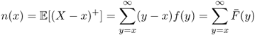
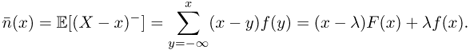
C.7 Partial Expectations
The following formulas computes partial expectations of a random variable with pdf f and cdf F. (If ![]() and
and ![]() , these each equal the true mean.)
, these each equal the true mean.)
Discrete versions are also available:


For a continuous random variable X and constants a and b, the identities above can be used to prove: