Chapter 13
The Bullwhip Effect
13.1 Introduction
In the early 1990s, executives at Procter & Gamble (P&G) noticed a peculiar trend in the orders for Pampers, a brand of baby diapers. As you might expect, demand for diapers at the consumer level is pretty steady since babies use them at a fairly constant rate. But P&G noticed that the orders placed by retailers (e.g., CVS, Target) to distributors were quite variable over time—high one week, low the next. The distributors' orders to P&G were even more variable, and P&G's orders to its own suppliers (e.g., 3M) were still more variable. (See Figure 13.1.)

Figure 13.1 Increase in order variability in upstream supply chain stages.
This phenomenon is known as the bullwhip effect (BWE), a phrase coined by P&G executives that refers to the way a wave's amplitude increases as it travels the length of a whip. Sometimes it's also known as the “whiplash” or “whipsaw” effect. The BWE has been observed in many industries other than diapers. For example, Hewlett‐Packard (HP) noticed large variability in the orders retailers placed to HP for printers, even though demand for printers is fairly steady. Similarly, the demand for DRAM (a component of computers) is more volatile than the demand for computers themselves. Wide swings in order sizes can cause big increases in inventory costs (for both raw materials and finished goods), overtime and idling expenses, and emergency shipment costs. These factors are estimated to increase costs by as much as 12.5–25% (Lee et al., 1997a).
The BWE was described in the literature as early as the 1950s (Forrester, 1958). Sterman (1989) described how the BWE could be caused by irrational behavior by supply chain managers: for example, overreacting to a small shortage one week by ordering far too much the next week. His paper uses the now‐famous “beer game” to demonstrate this relationship empirically. Then, two papers by Lee et al. (1997a,b) demonstrated that the BWE can occur even if all players act rationally—following the logical, optimized policies of the type we discuss in this book. They identified four primary causes for the BWE:
-
Demand signal processing. Many firms use forecasting techniques to estimate the mean and standard deviation of current or future demands. Each time a new demand is observed, the estimates are updated. If the previous period's demand was high, the new estimate will be higher than the previous one, thus raising the target inventory level. The orders will be more exaggerated than the demands. This phenomenon is amplified by the lead time if the base‐stock level is set using (4.46), that is,

where
 and
and  are the mean and standard deviation of the demand per period and L is the lead time. In practice, the firm doesn't know
  and
and  , so it estimates them based on historical data. These estimates change periodically, and any change in the estimates are magnified by the lead time when setting base‐stock levels, so long lead times produce large shifts in order sizes.
 -
Rationing game. When distributors don't have enough inventory to meet retailers' orders, they often allocate product according to order size: If retailer 1 orders 100 units and retailer 2 orders 150 units, but there are only 200 units available, then the distributor will give
 units to retailer 1 and
  units to retailer 2. If the retailers anticipate the shortage, they may artificially inflate their orders to try to get a larger allocation of the inventory. Once the shortage is over, the retailers' orders will return to their normal levels, or even lower. Thus, the variance in retailer orders is larger than the variance in actual demands.
 - Order batching. It is common for all players in a supply chain to place orders in bulk: Parents buy diapers in packages of 50, retailers buy them by the case, distributors buy them by the truckload. A theoretical explanation for the optimality of bulk ordering is that there is a fixed cost to place each order, so it's better to place fewer orders if possible. (For parents, the fixed cost is in the form of inconvenience and time: They don't want to go to the drug store every time their baby uses another diaper.) Moreover, bulk buying is encouraged by sellers by offering quantity discounts, another common practice. But order batching means that orders may be high one week, then low for the next few weeks as retailers use up the stock they've accumulated. Another reason for order batching is that many firms use material requirements planning (MRP) software that evaluates the firm's requirements for every part it uses and automatically places orders with suppliers once per month. That means the supplier sees large demand during a few days of the month as its customers' MRP systems place orders and small demand for the rest of the month; this is sometimes known as the “hockey stick” phenomenon.
- Price speculation. Prices change all the time, and firms tend to stock up while prices are low and order less when prices are high. This is most pronounced at upstream stages in the supply chain, whose raw materials are commodities such as plastic, steel, fuel, and so on—prices for these commodities change constantly, and speculation is common among buyers. It's also obvious at the other end of the supply chain, as customers buy more when retailers offer sales and promotions. In the middle of the supply chain, sales and promotions are common, too, causing retailers and other players to stock up when prices drop. All of this leads to large variability in buying patterns.
InSection 13.2, we'll discuss mathematical models explaining these causes and demonstrating that they occur even when each player in the supply chain is a rational “optimizer.” Then, in Section 13.3, we'll discuss strategies for reducing the BWE. Finally, in Section 13.4, we'll examine the extent to which sharing demand information with upstream supply chain members can reduce or eliminate the BWE.
Most of the analysis in this section is adapted from Lee et al. (1997a) and Chen et al. (2000). For reviews of the literature on the BWE, see McCullen and Towill (2002), Lee et al. (2004), or Geary et al. (2006).
13.2 Proving the Existence of the Bullwhip Effect
13.2.1 Introduction
Consider a serial supply chain like the one pictured in Figure 13.2. We will examine this system in the context of an infinite horizon under periodic review. Each stage places orders from its upstream stage and supplies product to its downstream stage. Stage N serves the end customer.
Our strategy will be to focus on one stage and to show that the variance of orders it places to its supplier is larger than the variance of orders it receives from its customer. That, in turn, implies the BWE as a whole: Stage N's orders are more variable than its demands, so stage ![]() 's orders are even more variable, so stage
's orders are even more variable, so stage ![]() 's orders are even more variable, and so on.
's orders are even more variable, and so on.

Figure 13.2 Serial supply chain network.
Suppose the following conditions hold at each stage:
- Demands are independent over time, and the parameters of the demand distribution are known.
- The stage's supplier (i.e., its upstream stage) always has sufficient inventory and satisfies orders with a fixed lead time that is independent of the order size.
- There is no fixed ordering cost.
- The purchase cost is constant over time.
If all four of these conditions hold, it is optimal for the stage to follow a stationary base‐stock policy. As we know from Section 4.3, that means that in each period, the order placed by the stage is exactly equal to the demand seen by the stage in the previous time period, so the orders placed by the stage and the demand seen by it have the same variance—the bullwhip effect does not occur.
However, relaxing each of the conditions given above (one at a time) gives us the four causes of the BWE: demand signal processing (when the demand parameters are unknown and hence forecasting techniques must be used to estimate them), rationing game (when supply is limited), order batching (when there is a fixed cost for ordering), and price speculation (when the purchase price can change over time).
We discuss models for each of these causes next. In each of the four sections that follows, we will consider only a single stage in the supply chain and show that the orders placed by the stage to its supplier have larger variance than the demands received by the stage. Without loss of generality we will refer to this stage as the “retailer.”
13.2.2 Demand SignalProcessing
In this section, we relax both parts of assumption #1 in Section 13.2.1: We assume that the demands are serially correlated—that is, demands in one time period are statistically dependent on demands in the previous time period—and that the parameters of the demand process are unknown and must be estimated. Each stage in the supply chain makes its own estimate of the demand parameters based on the orders it receives. We will show that this processing of the demand signal can lead to the BWE.
We assume that the demands seen by the retailer follow a first‐order autoregressive ![]() process; that is, the demand follows a model of the form
process; that is, the demand follows a model of the form
where ![]() is the demand in period t (a random variable),
is the demand in period t (a random variable), ![]() is a constant,
is a constant, ![]() is a correlation constant with
is a correlation constant with ![]() , and
, and ![]() is an error term that is distributed
is an error term that is distributed ![]() . If
. If ![]() is close to 1, then a large demand tends to be followed by another large demand, while if
is close to 1, then a large demand tends to be followed by another large demand, while if ![]() is close to
is close to ![]() , then a large demand tends to be followed by a small one.
, then a large demand tends to be followed by a small one.
It's tempting to think of d as the mean of this process, but it is not, unless ![]() . In fact, it can be shown that
. In fact, it can be shown that
Note that the mean, variance, and covariance are the same in every period. If ![]() , the demands are iid with mean d and variance
, the demands are iid with mean d and variance ![]() . These are steady‐state values; if we know
. These are steady‐state values; if we know ![]() , then these formulas do not apply. (See, for example, Problem 13.3.)
, then these formulas do not apply. (See, for example, Problem 13.3.)
The retailer follows a base‐stock policy. Let ![]() be the lead‐time demand for an order placed in period t; that is,
be the lead‐time demand for an order placed in period t; that is,

If the retailer knew the mean ![]() and standard deviation
and standard deviation ![]() of the lead‐time demand (which it could calculate if it knew d,
of the lead‐time demand (which it could calculate if it knew d, ![]() , and
, and ![]() —see Problem 13.3), then, analogous to (4.46), the optimal base‐stock level would be given by
—see Problem 13.3), then, analogous to (4.46), the optimal base‐stock level would be given by
However, the retailer does not know ![]() and
and ![]() but instead must forecast them based on observed demands using, for example, one of the methods in Chapter 2. One of the most common forecasting techniques, and the one we'll use here, is a moving average (Section 2.2.1), which simply consists of the average of the demands from the previous m time periods. The estimate for
but instead must forecast them based on observed demands using, for example, one of the methods in Chapter 2. One of the most common forecasting techniques, and the one we'll use here, is a moving average (Section 2.2.1), which simply consists of the average of the demands from the previous m time periods. The estimate for ![]() , computed at time t and denoted
, computed at time t and denoted ![]() , is
, is
As for the standard deviation, it turns out that instead of estimating the standard deviation of lead‐time demand (![]() ), we want to estimate the standard deviation of the forecast error of the lead‐time demand,
), we want to estimate the standard deviation of the forecast error of the lead‐time demand, ![]() . (See Section 4.3.2.7.) The estimate of
. (See Section 4.3.2.7.) The estimate of ![]() at time t is given by
at time t is given by
where
is the one‐period forecast error and ![]() is a constant depending on L,
is a constant depending on L, ![]() , and m; we omit the derivation of this equation and the exact form of
, and m; we omit the derivation of this equation and the exact form of ![]() . The base‐stock level is then set using
. The base‐stock level is then set using
This policy is optimal for iid normal demands (i.e., if ![]() ) and is approximately optimal otherwise. (It is only approximately optimal because these estimates of
) and is approximately optimal otherwise. (It is only approximately optimal because these estimates of ![]() and
and ![]() do not take into account the autocorrelation of the demand; that is, they assume that the demand will have the same distribution in each period of the lead time. It would be more accurate to account for the correlation, i.e., using 13.1, when estimating the lead‐time demand parameters. This is relatively straightforward to do if d,
do not take into account the autocorrelation of the demand; that is, they assume that the demand will have the same distribution in each period of the lead time. It would be more accurate to account for the correlation, i.e., using 13.1, when estimating the lead‐time demand parameters. This is relatively straightforward to do if d, ![]() , and
, and ![]() are known—see Problem 13.3—but is quite a bit harder when the parameters are unknown and are estimated as described above.)
are known—see Problem 13.3—but is quite a bit harder when the parameters are unknown and are estimated as described above.)
In period t, the retailer computes ![]() and
and ![]() using the previous m periods' demands, then sets the base‐stock level
using the previous m periods' demands, then sets the base‐stock level ![]() using 13.9 and places an order of size
using 13.9 and places an order of size ![]() (why?). (It is possible that
(why?). (It is possible that ![]() . In this case, we assume that the firm returns
. In this case, we assume that the firm returns
![]() units to the supplier and receives a full refund for the returned units.) We can write
units to the supplier and receives a full refund for the returned units.) We can write ![]() as
as

We want to compute ![]() so that we can compare it to
so that we can compare it to ![]() to demonstrate the BWE. Using the fact that
to demonstrate the BWE. Using the fact that
we have

Let's examine the ![]() term. Recall that
term. Recall that

Then

To evaluate this further, we'll need the following lemma:
Therefore, the first and last terms of 13.12 are equal to 0. As for the middle terms,

Therefore, we can ignore the ![]() term in 13.11. Then using 13.10 again, we have
term in 13.11. Then using 13.10 again, we have
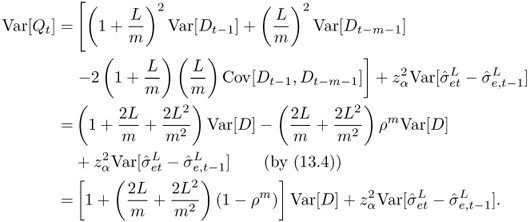
This gives us the following theorem:
Theorem 13.1 demonstrates that demand forecasting in the presence of positive lead times is sufficient to create the BWE at a single stage. Moreover, it provides a lower bound on the percentage increase in variability. For shorthand, let B equal the lower bound on ![]() , i.e., the right‐hand side of 13.13. Theorem 13.1 demonstrates that:
, i.e., the right‐hand side of 13.13. Theorem 13.1 demonstrates that:
- As m increases, B decreases. This is intuitive since larger m means smoother forecasts, so less variability in the order sizes.
- As L increases, B increases. This is also reasonable since longer lead times make it harder to forecast demand, so the forecasts themselves, and hence the order sizes, will be more variable.
- If
 (positively correlated demand), then as
  increases, B decreases. The intuitive explanation is that stronger positive correlation means there is more information available to make forecasts since each demand observation also provides information about past and future demands.
 - If
 (negatively correlated demand), then as
  increases, B decreases if m is even and increases if m is odd. At first it seems surprising that the directional change in B should depend on whether m happens to be odd or even, but here is an explanation. Suppose
  , so that the demand alternates between large and small values. If m is even, then the moving average always includes the same number of large and small values, so the forecast does not change much from period to period. On the other hand, if m is odd, then the moving average itself will alternate between large and small values. Therefore, B will be smaller if m is even than if it is odd, and the difference between these two cases will be more exaggerated as
  .
. - If
 , then the bound given in Theorem 13.1 is tight. In this case, no safety stock is held and stockouts occur in 50% of the periods. Simulation results given by Chen et al. (2000) suggest that even when
  , the bound given by the theorem is reasonably tight.
Theorem 13.1 establishes that the BWE occurs when the demand is autocorrelated and the parameters are unknown. In fact, either of these conditions, by itself, is sufficient to cause the BWE. If demands are independent over time (i.e., ![]() and the retailer knows this) but d and
and the retailer knows this) but d and ![]() are still unknown, then Theorem 13.1 still applies and
are still unknown, then Theorem 13.1 still applies and ![]() , so the BWE occurs. If, on the other hand, demands are still serially correlated but d,
, so the BWE occurs. If, on the other hand, demands are still serially correlated but d, ![]() , and
, and ![]() are known, then the BWE occurs as well; see Problem 13.4 or Zhang (2004).
are known, then the BWE occurs as well; see Problem 13.4 or Zhang (2004).
13.2.3 Rationing Game
Supposethe supply for a given product may be insufficient to meet the demand from multiple retailers and that the supplier will ration the available supply according to the fraction of demand accounted for by each retailer: If a retailer accounted for 8% of the total demand, it will receive 8% of the available supply. The BWE occurs when retailers anticipate the shortage since they have an incentive to inflate their orders to try to gain a larger share of the available supply. This behavior is called the rationing game because retailers play a “game” (in the game‐theory sense) to try to obtain a larger allocation in the face of the supplier's rationing.
We will consider the following simple model. There are two identical retailers, each facing demand with pdf ![]() and cdf
and cdf ![]() (the same distribution for both retailers). There is no inventory carryover between periods and unmet demands at the retailers are lost; therefore, we can model a single period and treat the multiperiod problem as multiple copies of the single‐period one. Each unit on hand at the end of a period incurs a cost of h, and each lost sale incurs a stockout penalty of p.
(the same distribution for both retailers). There is no inventory carryover between periods and unmet demands at the retailers are lost; therefore, we can model a single period and treat the multiperiod problem as multiple copies of the single‐period one. Each unit on hand at the end of a period incurs a cost of h, and each lost sale incurs a stockout penalty of p.
Let ![]() be the optimal order quantity if the supply were infinite; that is,
be the optimal order quantity if the supply were infinite; that is,
(from (4.17)). We assume that the available supply A can take on two quantities: It will equal ![]() with probability r and
with probability r and ![]() with probability
with probability ![]() , with
, with ![]() . That is, with probability r, there will be a supply shortage, and with probability
. That is, with probability r, there will be a supply shortage, and with probability ![]() , there will be adequate supply. (Lee et al. (1997a) consider a model with N retailers and a more general supply process, but the simpler model presented here conveys most of the same insights.)
, there will be adequate supply. (Lee et al. (1997a) consider a model with N retailers and a more general supply process, but the simpler model presented here conveys most of the same insights.)
If a retailer expects a supply shortage, it has an incentive to order more than ![]() . We will evaluate the Nash equilibrium solution—the order quantities chosen by the two retailers such that neither retailer, knowing the other's order quantity, would want to change its own. Put another way, a retailer's Nash equilibrium solution is the order quantity it chooses assuming it knows the other retailer's order quantity already.
. We will evaluate the Nash equilibrium solution—the order quantities chosen by the two retailers such that neither retailer, knowing the other's order quantity, would want to change its own. Put another way, a retailer's Nash equilibrium solution is the order quantity it chooses assuming it knows the other retailer's order quantity already.
Let ![]() be the order size for retailer i,
be the order size for retailer i, ![]() . If
. If ![]() , then retailer i will receive
, then retailer i will receive ![]() units. For convenience, define retailer 1's allocation as
units. For convenience, define retailer 1's allocation as
If ![]() is fixed, retailer 1's expected cost is given by
is fixed, retailer 1's expected cost is given by

The first term of 13.14 represents the expected cost when ![]() , while the second term assumes
, while the second term assumes ![]() . An analogous expression describes retailer 2's expected cost.
. An analogous expression describes retailer 2's expected cost.
Therefore, in the presence of supply shortages, order quantities will be inflated. However, this, by itself, does not prove that the BWE occurs in the rationing game, since inflated order quantities do not necessarily imply inflated variances. However, Lee et al. (1997a) argue that the theorem
…implies the bullwhip effect when the mean demand changes over time. Retailers' equilibrium order quantity may be identical or close to the newsvendor solution for low‐demand periods, while it will be larger than the newsvendor solution for high‐demand periods. Hence, the variance is amplified at the retailer.
It takes some additional work to prove this claim rigorously. In fact, it can be shown that, if the mean demand changes over time as described in the quote above, then there is no finite Nash equilibrium in the rationing game defined by Lee et al. (1997a). That is, the retailers will keep inflating their order quantities in response to one another ad infinitum. However, under some minor modifications, a Nash equilibrium does exist, and its variance is greater than that of the demand, as suggested in the quote. (See Rong et al. (2017b)for these results.)
13.2.4 Order Batching
Wewill model the batching of orders by assuming that a given retailer will not place an order in every time period. Instead, each retailer uses a periodic‐review base‐stock policy with a reorder interval of R periods—that is, every Rth period, the retailer places an order whose size is equal to the demand seen by the retailer in the previous R periods. (See Section 4.3.4.1.) If the supplier serves several retailers, we will show that the variance of the orders seen by the supplier is larger than the variance of the orders seen by the retailers.
Suppose that there are N retailers; retailer i sees a demand of ![]() in period t, with
in period t, with ![]() . Demands are independent among retailers and across time periods. We consider three cases corresponding to how the retailers' orders line up with one another: random ordering, positively correlated ordering, and balanced ordering.
. Demands are independent among retailers and across time periods. We consider three cases corresponding to how the retailers' orders line up with one another: random ordering, positively correlated ordering, and balanced ordering.
13.2.4.1 Random Ordering
Suppose each retailer's ordering period is chosen randomly from ![]() with equal probability. Let X be a random variable indicating the number of orders seen by the supplier in a given time period. Since each retailer orders with probability
with equal probability. Let X be a random variable indicating the number of orders seen by the supplier in a given time period. Since each retailer orders with probability ![]() in a given time period, X is a binomial random variable with parameters N and
in a given time period, X is a binomial random variable with parameters N and ![]() , and
, and

Let ![]() be the total size of the orders received by the supplier in period t. Without loss of generality, assume that retailers
be the total size of the orders received by the supplier in period t. Without loss of generality, assume that retailers ![]() are the retailers that order in period t and retailers
are the retailers that order in period t and retailers ![]() are the retailers that do not. Then
are the retailers that do not. Then

(The superscript r stands for “random.”) Then
where the notation ![]() means we take the expectation of
means we take the expectation of ![]() for fixed X, then take the expectation over X. Similarly,
for fixed X, then take the expectation over X. Similarly,

(The first equality is a well‐known identity for variance.) Therefore, the variance of orders seen by the supplier is greater than or equal to that of the demands seen by the retailers. Note that if ![]() (no order batching: every retailer orders every time period), the variances are equal, as expected.
(no order batching: every retailer orders every time period), the variances are equal, as expected.
13.2.4.2 Positively Correlated Ordering
We'll consider the extreme case in which all retailers order in the same period. For example, if R is 1 week, then all retailers order on Monday (say) and not on other days of the week. This is the MRP “hockey stick” taken to its extreme. The distribution function of X (the number of retailers ordering on a given day) is then

with

Let ![]() be the total size of the orders received by the supplier in period t. Then
be the total size of the orders received by the supplier in period t. Then
and

Again, the variance of orders is greater than the variance of demands, unless ![]() .
.
13.2.4.3 Balanced Ordering
Finally, suppose that the retailers' orders are evenly spread throughout the R‐period reorder interval. We'll write the number of retailers N as ![]() for integers M and k. M is like N
for integers M and k. M is like N
div
R and k is like N
mod
R. For example, if ![]() (1‐week reorder interval) and
(1‐week reorder interval) and ![]() , then
, then ![]() and
and ![]() . Three days a week, six retailers order, and four days a week, five retailers order. More generally, the retailers are divided into R groups, each ordering on a different day. k of the groups have size
. Three days a week, six retailers order, and four days a week, five retailers order. More generally, the retailers are divided into R groups, each ordering on a different day. k of the groups have size ![]() and
and ![]() of them have size M.
of them have size M.
We get:

Then

Let ![]() be the total size of the orders received by the supplier in period t. Then
be the total size of the orders received by the supplier in period t. Then
and

Once again, the variance of orders is greater than or equal to that of demands. If ![]() or
or ![]() , then exactly the same number of retailers place orders on each day, and the variances are equal.
, then exactly the same number of retailers place orders on each day, and the variances are equal.
We now have the following theorem.
Therefore, the orders placed to the supplier have the same mean as those placed to the retailers, but larger variance. Moreover, correlated demand produces the largest BWE, then random, then balanced.
13.2.5 Price Speculation
Wewill consider a single retailer whose supplier alternates between two prices, ![]() and
and ![]() , with
, with ![]() . With probability r, the price will be
. With probability r, the price will be ![]() and with probability
and with probability ![]() , the price will be
, the price will be ![]() . The long‐run expected discounted cost, over an infinite horizon, can be written recursively as a dynamic program (DP), similar to (4.36):
. The long‐run expected discounted cost, over an infinite horizon, can be written recursively as a dynamic program (DP), similar to (4.36):
where ![]() and, as usual,
and, as usual, ![]() is as given by (4.37). Note that we have two recursive functions, one for each cost level. The recursion 13.18 differs from (4.36) in two respects. First, the expected future cost contains an expectation over the cost level i. Second, this is an infinite‐horizon recursion, so
is as given by (4.37). Note that we have two recursive functions, one for each cost level. The recursion 13.18 differs from (4.36) in two respects. First, the expected future cost contains an expectation over the cost level i. Second, this is an infinite‐horizon recursion, so ![]() does not have a time‐period index, and the definition of
does not have a time‐period index, and the definition of ![]() depends on itself. Dynamic programming has tools to deal with this sort of recursion, which we will not explore here. Suffice it to say that the optimal inventory policy in this case can be shown to be a modified base‐stock policy: When the price is
depends on itself. Dynamic programming has tools to deal with this sort of recursion, which we will not explore here. Suffice it to say that the optimal inventory policy in this case can be shown to be a modified base‐stock policy: When the price is ![]() , order enough to bring the inventory position to
, order enough to bring the inventory position to ![]() , and when the price is
, and when the price is ![]() , order enough to bring the inventory position to
, order enough to bring the inventory position to ![]() . If the inventory level is greater than the applicable base‐stock level in a given period, returns are not allowed; instead, the retailer orders 0. It is clear that
. If the inventory level is greater than the applicable base‐stock level in a given period, returns are not allowed; instead, the retailer orders 0. It is clear that ![]() , but finding the optimal
, but finding the optimal ![]() and
and ![]() can be difficult. We omit the details here. The net result is the following theorem:
can be difficult. We omit the details here. The net result is the following theorem:
Therefore, price fluctuations produce the BWE.
You can get a feel for how this works by building a spreadsheet simulation model. For example, Figure 13.3 shows the first few rows of a spreadsheet that has columns for starting inventory, demand (we used ![]() to generate demand), price (low or high; we used
to generate demand), price (low or high; we used ![]() ), and order size (we used
), and order size (we used ![]() ,
, ![]() to compute these, but these are not the optimal base‐stock levels). The results of the simulation are displayed graphically in Figure 13.4. The orders clearly display a larger variance than the demands.
to compute these, but these are not the optimal base‐stock levels). The results of the simulation are displayed graphically in Figure 13.4. The orders clearly display a larger variance than the demands.

Figure 13.3 BWE spreadsheet simulation.

Figure 13.4 BWE caused by price fluctuations.
13.3 Reducing the Bullwhip Effect
A number of strategies have been proposed for addressing the four causes of the BWE. We discuss some of these next.
13.3.1 Demand Signal Processing
The analysis given above suggests that the BWE is amplified as we move upstream in the supply chain since stage i uses stage ![]() 's orders as though they were demands, when in fact they are more variable than demands. This can be mitigated by sharing point‐of‐sale (POS) demand information with upstream members of the supply chain. That is, when the retailer places an order with the wholesaler, it relays not only the order size but also the size of the most recent demands. The proliferation of bar code scanners at checkout lines makes this technologically easy, but retailers are often reluctant to give demand data, which they treat as proprietary, to their suppliers. In addition, even if upstream stages see this “sell‐through” data, they may each use different forecasting techniques or inventory policies, and this will exacerbate the BWE as well. We will analyze the effect of sell‐through data on the BWE in Section 13.4.
's orders as though they were demands, when in fact they are more variable than demands. This can be mitigated by sharing point‐of‐sale (POS) demand information with upstream members of the supply chain. That is, when the retailer places an order with the wholesaler, it relays not only the order size but also the size of the most recent demands. The proliferation of bar code scanners at checkout lines makes this technologically easy, but retailers are often reluctant to give demand data, which they treat as proprietary, to their suppliers. In addition, even if upstream stages see this “sell‐through” data, they may each use different forecasting techniques or inventory policies, and this will exacerbate the BWE as well. We will analyze the effect of sell‐through data on the BWE in Section 13.4.
Vendor‐managed inventory (VMI) is a distribution strategy whereby the vendor (say, Coca‐Cola) manages the inventory at the retailer (say, Walmart). The Coca‐Cola company sets up the Coke displays at Walmart and, more importantly, monitors the inventory level and replenishes as necessary. In many cases, Coke actually owns the merchandise until it is sold—Walmart only takes ownership of the product for a split second as it's being scanned at the checkout line. Walmart benefits because Coke pays some of the costs of holding and managing the inventory. Coke benefits because it can keep tighter control over the displays of its products at stores, and also because its distribution is more efficient when it, not its customers, decides when to replenish the stock at each store. Moreover, since Coke gets to see actual sales data, the BWE is reduced.
As we saw earlier, longer lead times make the BWE worse. Therefore, one strategy for reducing the BWE is to shorten lead times. There are various ways to accomplish this, though it is often easier said thandone.
13.3.2 Rationing Game
Ratherthan rationing according to order sizes in the current period, the supplier could allocate the available supply based on each retailer's orders in the previous period, or based on market share or some other mechanism that's independent of this period's orders. That eliminates the incentive to over‐order during shortages. Alternatively, the supplier could restrict each retailer's orders to be no more than a certain percentage (say 10%) larger than its order in the previous period, or charge a small “reservation payment” for each item ordered, whether or not it is received. Finally, the supplier can avoid the rationing game to a certain extent by sharing supply information with downstream members (note the symmetry with the demand signal processing case), allowing the retailers to use actual data instead of conjecture when making orderingdecisions.
13.3.3 Order Batching
Recallfrom the EOQ model (Section 3.2) that as the fixed order cost increases, so does the order size. The batching of orders, then, can be reduced by reducing the fixed order cost. Nowadays, most communication uses electronic data interchange (EDI), in which communication is performed electronically instead of on paper. This reduces the cost in both time and money of placing each order. Another innovation that reduces the setup cost of each order is third‐party logistics (3PL) providers, which allow smaller companies to attain larger economies of scale by taking advantage of the 3PL's size. For example, if a firm wants to ship a single package to a customer, it doesn't have to contract for a full truck—it can just use UPS, one of the world's largest 3PLs. Since UPS has lots of packages going all over the world, it attains huge economies of scale and passes some of these savings to its customers.
Suppliers can also encourage less batching by offering retailers volume discounts based on their total order, not based on orders for individual products. For example, P&G used to give bulk discounts if retailers ordered an entire truckload of one product (say, Pampers); now they give the same discounts even if the truck carries a variety of P&G products. This allows retailers to order Pampers more frequently (possibly with every order) as opposed to only ordering Pampers when they need a full truckload.
If batching is unavoidable, suppliers can force the orders to be balanced over time by assigning each retailer a specific period during which it may place orders. For example, one retailer might have to place orders only on Tuesdays, while another may place orders on Thursdays. This strategy will reduce, but not avoid, the BWE, as we sawin Theorem 13.3.
13.3.4 Price Speculation
Oneway to avoid the variability introduced by price fluctuations is simply to keep prices fixed. Although this seems obvious, it has introduced a shift in the pricing schemes of many major manufacturers such as P&G, Kraft, and Pillsbury. The strategy is called everyday low pricing (EDLP), and the basic idea is that prices stay at a constant low rate: there are no sales or promotions. EDLP is widely used upstream in the supply chain, but it is also increasingly used for retail sales. You may have seen stores that advertise “everyday low prices” and assumed it is merely a marketing ploy, without realizing the substantial benefit the retailer may be gaining by reducing the BWE.
In some cases, price fluctuations are unavoidable or desirable, and a natural consequence is that retailers will buy more when the price is low. The supplier can still reduce the BWE, however, by proposing contracts in which the retailer agrees to buy a large quantity of goods at a discount but to spread the receipt of the goods over time. The manufacturer can plan production more efficiently, but the retailer can continue to buy when pricesare low.
13.4 Centralizing Demand Information
InSection 13.3, we suggested that sharing POS demand information with upstream supply chain members reduces the BWE: Instead of seeing the retailer's orders, which are already more variable than the demands, the supplier sees the actual demands and uses these to make its own ordering decisions. But can this strategy eliminate the BWE entirely? If not, how much can it reduce the BWE?
In this section, we will analyze the impact of demand sharing on the BWE using the model introduced in Section 13.2.2, extending the analysis now to multiple stages as pictured in Figure 13.2. We will consider a centralized system in which each stage sees the actual customer demands; we will then compare this system to a decentralized system in which demand information is not shared and each stage sees only the orders placed by its immediate downstream neighbor.
The lead time for goods being transported from stage i to stage ![]() is given by
is given by ![]() . Each stage uses a moving average forecast with m observations. The moving average is used to compute estimates of the lead time demand mean,
. Each stage uses a moving average forecast with m observations. The moving average is used to compute estimates of the lead time demand mean, ![]() , and the standard deviation of the forecast error of lead‐time demand,
, and the standard deviation of the forecast error of lead‐time demand,![]() , which are in turn used to compute the base‐stock levels.
, which are in turn used to compute the base‐stock levels.
13.4.1 Centralized System
In the centralized system, demand information is available to all stages of the supply chain. There is no “information lead time”—all stages see customer demands at exactly the same moment, when the demands arrive. Stage i can build its moving average forecast using actual customer demands. Its estimates of ![]() and
and ![]() will be as given in 13.7 and 13.8, and it will use these to compute base‐stock levels as in 13.9.
will be as given in 13.7 and 13.8, and it will use these to compute base‐stock levels as in 13.9.
Conceptually, there is no difference between (a) goods being shipped from i to ![]() to … to N to the customer, with a total lead time of
to … to N to the customer, with a total lead time of ![]() , and (b) goods being shipped directly from i to the customer with the same lead time. Therefore, we can think of stage i as serving the end customer demand directly with a transportation lead time of
, and (b) goods being shipped directly from i to the customer with the same lead time. Therefore, we can think of stage i as serving the end customer demand directly with a transportation lead time of ![]() . Using the same logic as in Section 13.2, we get the following theorem, which quantifies the increase in variability between the customer demands and the orders placed by a given stage:
. Using the same logic as in Section 13.2, we get the following theorem, which quantifies the increase in variability between the customer demands and the orders placed by a given stage:
Thus, even if (1) demand information is visible to all supply chain members, (2) all supply chain members use the same forecasting technique, and (3) all supply chain members use the same inventory policy, the bullwhip effect still exists. Sharing demand information does not eliminate the BWE. But does it reduce it? We will answer this question in the next section by comparing this system to one in which demand information is not shared.
13.4.2 Decentralized System
Consider the same system as in the previous section except that demand information is not shared: Each stage only sees the orders placed by its downstream stage. For simplicity, we will assume that ![]() (demands are uncorrelated across time). We will also assume that
(demands are uncorrelated across time). We will also assume that ![]() (a 50% service level is acceptable), which means no safety stock is held. (Firms sometimes use inventory policies of this form, inflating
(a 50% service level is acceptable), which means no safety stock is held. (Firms sometimes use inventory policies of this form, inflating ![]() artificially to provide a buffer against uncertainty. For example, the firm might increase
artificially to provide a buffer against uncertainty. For example, the firm might increase ![]() by 7 days, requiring 7 extra days of supply of inventory to be on hand at any given time. Firms generally refer to this inflated lead time as safety lead time, but we can think of safety lead time as essentially an alternate method of setting safety stock.)
by 7 days, requiring 7 extra days of supply of inventory to be on hand at any given time. Firms generally refer to this inflated lead time as safety lead time, but we can think of safety lead time as essentially an alternate method of setting safety stock.)
The “demands” seen by stage i are really the orders placed by stage ![]() . The variance of these orders is at least
. The variance of these orders is at least ![]() times the variance of the orders received by stage
times the variance of the orders received by stage ![]() , by Theorem 13.1. By following this logic through to stage N, we get the following theorem:
, by Theorem 13.1. By following this logic through to stage N, we get the following theorem:
Therefore, the increase in variability is additive in the centralized system but multiplicative in the decentralized system. Sharing demand information can significantly reduce the BWE. Although our analysis of the decentralized system assumed ![]() , the qualitative result (additive vs. multiplicative variance increase) still holds in the more general case, though the math is uglier.
, the qualitative result (additive vs. multiplicative variance increase) still holds in the more general case, though the math is uglier.
To get a sense of the difference in magnitude between the bounds provided by Theorems 13.5 and 13.6, consider the case in which ![]() ,
, ![]() for all i, and
for all i, and ![]() . Then the right‐hand sides of the inequalities are given in Table 13.1. Note how much larger the bounds are for the decentralized system, especially as we move upstream in the supply chain.
. Then the right‐hand sides of the inequalities are given in Table 13.1. Note how much larger the bounds are for the decentralized system, especially as we move upstream in the supply chain.
Table 13.1 Bounds on variability increase: Decentralized vs. centralized.
| i | Decentralized | Centralized |
| 1 | 12.7 | 7.2 |
| 2 | 6.7 | 5.0 |
| 3 | 3.6 | 3.2 |
| 4 | 1.9 | 1.9 |
PROBLEMS
- 13.1 (Stochastic Price Simulation) Suppose that the price of the raw material for a given product is stochastic, as in Section 13.2.5. The price equals
 with probability 0.8 and equals
  with probability 0.2. Demands in each period are
  . On‐hand inventory at the end of each period incurs a holding cost of
  per unit. Unmet demands are backordered with a stockout cost of
  per unit.
 The firm uses two base‐stock levels,
 and
and  , ordering up to the appropriate level in each period based on the current price. For now, assume
  and
and  .
.- Simulate this system using spreadsheet software for 1000 periods. Build a table like the one in Figure 13.3 listing the time period, starting inventory, demand, price, order size, and any other columns you find useful. Also indicate the total cost in each period, including holding, stockout, and order costs.
- Using a spreadsheet‐based nonlinear optimization package, determine the values of
 and
and  that minimize the average cost per period for the random sample you have generated. Report the optimal
  and
and  and the resulting average cost per period. Include the first few rows of your spreadsheet in your report.
 - Calculate
 and
and  for your simulation and compare them to verify that the BWE occurs.
 - Produce a chart like the one in Figure 13.4 plotting the demands and orders across the time horizon.
- 13.2 (Batching Simulation) In the one‐warehouse, multiple‐retailer (OWMR) system pictured in Figure 13.6, all three retailers, and the warehouse, handle a single product. Demands at the retailers are normally distributed with means and variances as given in Table 13.2, which also lists h, p, and K at each retailer. (As usual, h is the holding cost per item per period, p is the backorder cost per item per period, and K is the fixed cost per order placed to the warehouse.) Since
 , it's optimal for the retailers to follow an
  policy rather than a base‐stock policy.
- Compute near‐optimal values for s and S for each retailer using the power approximation from Section 4.4.4.
- Simulate this system using a spreadsheet or other software package using the
 values you found in part (a). Simulate at least 1000 periods, with a warm‐up interval of 100 periods. Report the standard deviation of the total demands seen by the retailers and the standard deviation of the total demands (retailer orders) seen by the warehouse. Using these values, verify that the BWE occurs in this system.
 - In a short paragraph, explain why the retailers'
 policies cause the BWE.

Figure 13.6 One‐warehouse, multiple‐retailer system for Problem 13.2.
Table 13.2 Data for Problem 13.2.
Retailer 

h p K 1 50 
0.6 7 100 2 100 
0.4 8 100 3 40 
0.9 4 100 - 13.3 (Lead‐Time Demand Under Autocorrelation) For the demand process in Section 13.2.2, prove that
 is normally distributed with mean
and standard deviation

(Note that
 is independent of t.)
 - 13.4 (BWE Occurs Even If Demand Parameters Are Known) Suppose that we know d,
 , and
, and  in Section 13.2.2. Using the results in Problem 13.3, prove that
(Since this is greater than 1, the BWE occurs even if the parameters are known and therefore no forecasting is required.)
- 13.5 (Proving BWE in the Beer Game) In the “stationary beer game” (Chen and Samroengraja, 2000), a serial supply chain faces normally distributed demands at the downstream node, and each stage orders from its supplier in each period. The optimal inventory policy at each stage is a base‐stock policy: The size of the order a stage places in a given period is equal to the size of the order received by the stage in that period. If each player followed this policy, there would be no BWE since the variance of outgoing orders would be the same as that of incoming orders. The beer game is designed to illustrate the irrational behavior of supply chain managers, who tend to over‐react to perceived trends in demand (even when no actual trend is present) by ordering more than necessary when demands are high and less than necessary when demands are low. In this problem, you will model this over‐reaction mathematically and prove that it causes the bullwhip effect.
Consider a retailer who faces demand
 in period t. Demands are independent across time periods. The retailer, acting irrationally, over‐orders by
  units for each consecutive period in which the demand was higher than
  , including the current period. Similarly, it under‐orders by
  units for each consecutive period in which the demand was lower than
  , where
  is a constant. That is, although the optimal policy is to set the order size as
  , the retailer actually uses
where
 is the number of consecutive periods (including t) in which the demand was greater than
  and
and  is the number of consecutive periods (including t) in which the demand was less than
  .
.- Prove that
 (the retailer's mean order size is equal to the mean demand).
 - Prove that

Hint 1: What probability distribution describes
 and
and  ?
?Hint 2: Remember that
 .
.
- Prove that
- 13.6 (Beer Game Simulation) In the beer game, players act irrationally (i.e., not following the optimal inventory policy). One model of this irrational behavior is by Sterman (1989), who suggests that the order quantity placed by stage i (
 ) in period t of the beer game can be described by the following model:
where
-
 ,
,  ,
,  , and
, and  are constants for stage i, described in more detail below
 -
 inventory level (on‐hand inventory minus backorders) at stage i after step 2 in the sequence of events given below (i.e., after observing its demand but before placing its order) in period t
-
 inventory position (on‐hand inventory plus on‐order inventory minus backorders) at stage i after step 2 in period t
-
 order quantity placed by stage i in step 3 in period t; if
  , then
  represents demand from the external customer
 -
 forecast of order quantity that will be placed by stage i in period t; this forecast is calculated by stage
  after step 2 in period
  using exponential smoothing:
where
 is the smoothing factor,
  .
.
The constants
 and
and  represent target values for the inventory level (
 ) and on‐order inventory (
 ), respectively, for stage i. The constants
  and
and  are adjustment parameters controlling the change in order quantity when the actual inventory level and the on‐order inventory, respectively, deviate from the desired targets.
The sequence of events at stage i in each period of the beer game is as follows:
- The shipment from stage
 shipped two periods ago arrives at stage i. (If
  , stage
  refers to the manufacturing process at the farthest upstream stage.)
 - The order placed by stage
 in the current period is observed by stage i. (If
  , stage
  refers to the external customer.) The order from stage
  , plus any backorders that stage
  is waiting for, is satisfied using the current on‐hand inventory, and excess demands are backordered.
 - Stage i determines its order quantity and places its order to stage
 .
. - Holding and/or stockout costs are incurred.
- Using MATLAB, Excel, or any other software package of your choice, simulate the beer game under the assumption that all players use 13.19 to set their order quantities. Assume that
 . Model the demand from the external customer in each period as an iid random variable distributed as
  . Set
. Set  ,
,  ,
,  , and
, and  for all i. Initialize the system by assuming that
  and
and  for all i, and that there are 50 units of in‐transit inventory due to arrive in each of period 1 and period 2 for each i. (That is, assume that each stage has 1 period's worth of inventory on‐hand and in each in‐transit slot.) Report the magnitude of the BWE at each stage, defined as
  .
. - Conduct a numerical experiment to evaluate how the BWE changes as the players' order behavior changes. At a minimum, use your experiment to answer the following questions:
- Does the BWE get more or less severe when stages increase the weight
 they place on the on‐hand inventory level?
 - Does the BWE get more or less severe when stages increase the weight
 they place on the on‐order inventory?
 - Does the BWE get more or less severe when stages increase their target levels
 and
and  ?
? - Does the BWE get more or less severe when stages increase the smoothing constant
 ?
? - Suppose stage i uses 13.19 to set order quantities but all other players are more rational, setting
 . Which produces more severe BWE—having the “irrational” player upstream or downstream in the supply chain?
Support your analysis with numerical results, preferably in graph (chart) form.
- Does the BWE get more or less severe when stages increase the weight
-