
Chapter 8
Facility Location
Models
8.1 Introduction
One of the major strategic decisions faced by firms is the number and locations of factories, warehouses, retailers, or other physical facilities. This is the purview of a large class of models known as facility location problems. The key trade‐off in most facility location problems is between the facility cost and customer service. If we open a lot of facilities (Figure 8.1(a)), we incur high facility costs (to build and maintain them), but we can provide good service since most customers are close to a facility. On the other hand, if we open few facilities (Figure 8.1(b)), we reduce our facility costs but must travel farther to reach our customers (or they to reach us).

Figure 8.1 Facility location configurations. Squares represent facilities; circles represent customers.
Most (but not all) location problems make two related sets of decisions: (1) where to locate, and (2) which customers are assigned or allocated to which facilities. Therefore, facility location problems are also sometimes known as location–allocation problems.
A huge range of approaches has been considered for modeling facility location decisions. These differ in terms of how they model facility costs (for example, some include the costs explicitly, while others impose a constraint on the number of facilities to be opened) and how they model customer service (for example, some include a transportation cost , while others require all or most facilities to be covered—that is, served by a facility that is within some specified distance). Facility location problems come in a great variety of flavors based on what types of facilities are to be located, whether the facilities are capacitated, which (if any) elements of the problem are stochastic, what topology the facilities may be located on (e.g., on the plane, in a network, or at discrete points), how distances or transportation costs are measured, and so on. Several excellent textbooks provide additional material for the interested reader; for example, see Mirchandani and Francis (1990), Drezner (1995a), Drezner and Hamacher (2002), or Daskin (2013). For an annotated bibliography of papers on facility location problems, see ReVelle et al. (2008b). The book by Eiselt and Marianov (2011) contains chapters on a number of seminal papers in facility location, each describing the original contribution as well as later extensions.
In addition to supply chain facilities such as plants and warehouses, location models have been applied to public sector facilities such as bus depots and fire stations, as well as to telecommunications hubs, satellite orbits, bank accounts, and other items that are not really “facilities” at all. In addition, many operations research problems can be formulated as facility location problems or have subproblems that resemble them. Facility location problems are often easy to state and formulate but are difficult to solve; this makes them a popular testing ground for new optimization tools. For all of these reasons, facility location problems are an important topic in operations research, and in supply chain management in particular, in both theoretical and applied work.
In this chapter, we will begin by discussing a classical facility location model, the uncapacitated fixed‐charge location problem (UFLP), in Section 8.2. The UFLP and its descendants have been deployed more widely in supply chain management than perhaps any other location model. One reason for this is that the UFLP is very flexible and, although it is NP‐hard, lends itself to a variety of effective solution methods. Another reason is that the UFLP includes explicit costs for both key elements of the problem—facilities and customer service—and is therefore well suited to supply chain applications.
In Section 8.3, we discuss other so‐called minisum models (in particular, the p‐median problem and a capacitated version of the UFLP), and in Section 8.4, we discuss covering models (including the p‐center, set covering, and maximal covering problems). We briefly discuss a variety of other deterministic facility location problems in Section 8.5. In Section 8.6, we introduce stochastic and robust models for facility location under uncertainty. We then discuss models for network design—a close cousin of facility location—in Section 8.7.
8.2 The Uncapacitated Fixed‐Charge Location Problem
8.2.1 Problem Statement
The uncapacitated fixed‐charge location problem (UFLP) chooses facility locations in order to minimize the total cost of building the facilities and transporting goods from facilities to customers. The UFLP makes location decisions for a single echelon, and the facilities in that echelon are assumed to serve facilities in a downstream echelon, all of whose locations are fixed. We will tend to refer to the facilities in the upstream echelon as distribution centers (DCs) or warehouses and to those in the downstream echelons as customers. However, the model is generic, and the two echelons may instead contain other types of facilities—for example, factories and warehouses, or regional and local DCs, or even fire stations and homes. Sometimes it's also useful to think of an upstream echelon, again with fixed location(s), that serves the DCs.
Each potential DC location has a fixed cost that represents building (or leasing) the facility; the fixed cost is independent of the volume that passes through the DC. There is a transportation cost per unit of product shipped from a DC to each customer. There is a single product. The DCs have no capacity restrictions—any amount of product can be handled by any DC. (We'll relax this assumption in Section 8.3.1.) The problem is to choose facility locations to minimize the fixed cost of building facilities plus the transportation cost to transport product from DCs to customers, subject to constraints requiring every customer to be served by some open DC.
As noted above, the key trade‐off in the UFLP is between fixed and transportation costs. If too few facilities are open, the fixed cost is small, but the transportation cost is large because many customers will be far from their assigned facility. On the other hand, if too many facilities are open, the fixed cost is large, but the transportation cost is small. The UFLP tries to find the right balance, and to optimize not only the number of facilities, but also their locations.
8.2.2 Formulation
Define the following notation:
| Sets | |
| I | = set of customers |
| J | = set of potential facility locations |
| Parameters | |
|
|
= annual demand of customer |
|
|
= cost to transport one unit of demand from facility |
|
|
= fixed annual cost to open a facility at site |
| Decision Variables | |
|
|
= 1 if facility j is opened, 0 otherwise |
|
|
= the fraction of customer i's demand that is served by facility j |
The transportation costs
![]() might be of the form
might be of the form ![]() for some constant k (if the shipping company charges k per mile per unit) or may be more arbitrary (for example, based on airline ticket prices, which are not linearly related to distance). In the former case, distances
may be computed in a number of ways:
for some constant k (if the shipping company charges k per mile per unit) or may be more arbitrary (for example, based on airline ticket prices, which are not linearly related to distance). In the former case, distances
may be computed in a number of ways:
-
Euclidean distance: The
distance between
 and
and  is given by
The Euclidean distance metric is also known as the
 norm. This is an intuitive measure of distance but is not usually applicable in supply chain contexts because Cartesian coordinates are not useful for describing real‐world locations.
 -
Manhattan or rectilinear metric: The
distance is given by

This metric assumes that travel is only possible parallel to the x‐ or y‐axis, e.g., travel along city streets. It is also known as the
 norm.
norm. -
Great circle: This
method for calculating distances takes into account the curvature of the earth and, more importantly, takes latitudes and longitudes as inputs and returns distances in miles or kilometers. Great circle distances assume that travel occurs over a great circle, the shortest route over the surface of a sphere. Let
 and
and  be the latitude and longitude of two points in radians, and let
  and
and  be the differences in the latitude and longitude (respectively). Then the great circle distance between the two points is given by
where r is the radius of the Earth, approximately 3958.76 miles or 6371.01 km (on average), and the trigonometric functions are assumed to use radians.
A simpler formula, known as the spherical law of cosines , sets the distance equal to
and is nearly as accurate as 8.1 except when the distance between the two points is very small. (See Problem 8.44.)
- Highway/network: The distance is computed as the shortest path within a network, for example, the US highway network. This is usually the most accurate method for calculating distances in a supply chain context. However, since they require data on the entire road network, they must be obtained from geographic information systems (GIS) or from online services such as Mapquest or Google Maps. (In contrast, the distance measures above can be calculated from simple formulas using only the coordinates of the facilities and customers.)
- Matrix: Sometimes a matrix containing the distance between every pair of points is given explicitly. This is the most general measure, since all others can be considered a special case. It is also the only possible measure when the cost structure exhibits no particular pattern—for example, when they are based on airline ticket prices.

In general, we won't be concerned with how transportation costs are computed—we'll assume they are given to us already as the parameters ![]() .
.
The UFLP is formulated as follows:
Formulations very similar to this were originally proposed by Manne (1964) and Balinski (1965). The objective function 8.3 computes the total (fixed plus transportation) cost. In the discussion that follows, we'll use ![]() to denote the optimal objective value of (UFLP). Constraints 8.4 require the full amount of every customer's demand to be assigned, to one or more facilities. These are often called assignment constraints. Constraints 8.5 prohibit a customer from being assigned to a facility that has not been opened. These are often called linking constraints. Constraints 8.6 require the location (x) variables to be binary, and constraints 8.7 require the assignment (y) variables to be nonnegative.
to denote the optimal objective value of (UFLP). Constraints 8.4 require the full amount of every customer's demand to be assigned, to one or more facilities. These are often called assignment constraints. Constraints 8.5 prohibit a customer from being assigned to a facility that has not been opened. These are often called linking constraints. Constraints 8.6 require the location (x) variables to be binary, and constraints 8.7 require the assignment (y) variables to be nonnegative.
Constraints 8.4 and 8.7 together ensure that ![]() . In fact, it is always optimal to assign each customer solely to its nearest open facility. (Why?) Therefore, there always exists an optimal solution in which
. In fact, it is always optimal to assign each customer solely to its nearest open facility. (Why?) Therefore, there always exists an optimal solution in which ![]() for all
for all ![]() . It is therefore appropriate to think of the
. It is therefore appropriate to think of the ![]() as binary variables and to talk about “the facility to which customer i is assigned.”
as binary variables and to talk about “the facility to which customer i is assigned.”
Another way to write constraints 8.5 is
If ![]() , then
, then ![]() can be 1 for any or all
can be 1 for any or all ![]() , while if
, while if ![]() , then
, then ![]() must be 0 for all i. These constraints are equivalent to 8.5 for the IP. But the LP relaxation
is weaker (i.e., it provides a weaker bound) if constraints 8.8 are used instead of 8.5. This is because there are solutions that are feasible for the LP relaxation with 8.8 that are not feasible for the LP relaxation with 8.5. To take a trivial example, suppose there are 2 facilities and 10 customers with equal demand, and suppose each facility serves 5 customers in a given solution. Then it is feasible to set
must be 0 for all i. These constraints are equivalent to 8.5 for the IP. But the LP relaxation
is weaker (i.e., it provides a weaker bound) if constraints 8.8 are used instead of 8.5. This is because there are solutions that are feasible for the LP relaxation with 8.8 that are not feasible for the LP relaxation with 8.5. To take a trivial example, suppose there are 2 facilities and 10 customers with equal demand, and suppose each facility serves 5 customers in a given solution. Then it is feasible to set ![]() for the problem with 8.8 but not with 8.5. Since the feasible region for the problem with 8.8 is larger than that for the problem with 8.5, its objective value is no greater. It is important to understand that the IPs have the same optimal objective value, but the LPs have different values—one provides a weaker LP bound than the
other.
for the problem with 8.8 but not with 8.5. Since the feasible region for the problem with 8.8 is larger than that for the problem with 8.5, its objective value is no greater. It is important to understand that the IPs have the same optimal objective value, but the LPs have different values—one provides a weaker LP bound than the
other.
The UFLP is NP‐hard (Garey and Johnson, 1979). A large number of solution methods have been proposed in the literature over the past several decades, both exact algorithms and heuristics. Some of the earliest exact algorithms involve simply solving the IP using branch‐and‐bound. Today, this would mean solving (UFLP) as‐is using CPLEX, Gurobi, or another off‐the‐shelf IP solver, although such general‐purpose solvers did not exist when the UFLP was first formulated. This approach works quite well using modern solvers, in part because the LP relaxation of (UFLP) is usually extremely tight, and in fact it often results in all‐integer solutions “for free” (Morris, 1978). (ReVelle and Swain (1970) discuss this property in the context of a related problem, the p‐median problem. ) Current versions of CPLEX or Gurobi can solve instances of the UFLP with thousands of potential facility sites in a matter of minutes. However, when it was first proposed that branch‐and‐bound be used to solve the UFLP (by Efroymson and Ray (1966)), IP technology was much less advanced, and this approach could only be used to solve problems of modest size. Therefore, a number of other optimal approaches were developed. Two of these—Lagrangian relaxation and a dual‐ascent method called DUALOC—are discussed in Sections 8.2.3 and 8.2.4, respectively. Many other IP techniques, such as Dantzig–Wolfe or Benders decomposition, have also been successfully applied to the UFLP (e.g., Balinski (1965) and Swain (1974)). We discuss heuristic methods for the UFLP in Section 8.2.5.
8.2.3 Lagrangian Relaxation
8.2.3.1 Introduction
One of the methods that has proven to be most effective for the UFLP and other location problems is Lagrangian relaxation, a standard technique for integer programming (as well as other types of optimization problems). The basic idea behind Lagrangian relaxation is to remove a set of constraints to create a problem that's easier to solve than the original. But instead of just removing the constraints, we include them in the objective function by adding a term that penalizes solutions for violating the constraints. This process gives a lower bound on the optimal objective value of the UFLP, but it does not necessarily give a feasible solution. Feasible solutions must be found using some other method (to be described below); each feasible solution provides an upper bound on the optimal objective value. When the upper and lower bounds are close (say, within 1%), we know that the feasible solution we have found is close to optimal.
For more details on Lagrangian relaxation, see Appendix D.1. See also Fisher (1981,1985) for excellent overviews. Lagrangian relaxation was proposed as a method for solving a UFLP‐like problem by Cornuejols et al. (1977).
We want to use Lagrangian relaxation on the UFLP formulation given in Section 8.2.2. The question is, which constraints should we relax? There are only two options: 8.4 and 8.5. (Constraints 8.6 and 8.7 can't be relaxed using Lagrangian relaxation.) Relaxing either 8.4 or 8.5 results in a problem that is quite easy to solve, and both relaxations produce the same bound (for reasons discussed below). But relaxing 8.4 involves relaxing fewer constraints, which is generally preferable (also for reasons that will be discussed below). Therefore, we will relax constraints 8.4, although in Section 8.2.3.8 we will briefly discuss what happens when constraints 8.5 are relaxed.
8.2.3.2 Relaxation
We relax constraints 8.4, removing them from the problem and adding a penalty term to the objective function:

The ![]() are called Lagrange multipliers.
There is one for each relaxed constraint. Their purpose is to ensure that violations in the constraints are penalized by just the right amount—more on this later. We'll use
are called Lagrange multipliers.
There is one for each relaxed constraint. Their purpose is to ensure that violations in the constraints are penalized by just the right amount—more on this later. We'll use ![]() to represent the vector of
to represent the vector of ![]() values.
values.
For now, assume ![]() is fixed. Relaxing constraints 8.4 gives us the following problem, known as
the Lagrangian subproblem:
is fixed. Relaxing constraints 8.4 gives us the following problem, known as
the Lagrangian subproblem:

(The subscript ![]() on the problem name reminds us that this problem depends on
on the problem name reminds us that this problem depends on ![]() as a parameter.) Since the
as a parameter.) Since the ![]() are all constants, the last term of 8.9 can be ignored during the optimization.
are all constants, the last term of 8.9 can be ignored during the optimization.
How can we solve this problem? It turns out that the problem is quite easy to solve by inspection—we don't need to use an IP solver or any sort of complicated algorithm. Suppose that we set ![]() for a given facility j. By constraints 8.10, setting
for a given facility j. By constraints 8.10, setting ![]() allows
allows ![]() to be set to 1 for any
to be set to 1 for any ![]() . For which i would
. For which i would ![]() be set to 1 in an optimal solution to the problem? Since this is a minimization problem,
be set to 1 in an optimal solution to the problem? Since this is a minimization problem, ![]() would be set to 1 for all i such that
would be set to 1 for all i such that ![]() . So if
. So if ![]() were set to 1, the benefit (or contribution to the objective function) would be
were set to 1, the benefit (or contribution to the objective function) would be
Now the question is, which ![]() should be set to 1? It's optimal to set
should be set to 1? It's optimal to set ![]() if and only if
if and only if ![]() ; that is, if the benefit of opening the facility outweighs its fixed cost. Theorem 8.1 summarizes these conclusions.
; that is, if the benefit of opening the facility outweighs its fixed cost. Theorem 8.1 summarizes these conclusions.
Notice that in optimal solutions to (UFLP‐LRλ), customers may be assigned to 0 or more than 1 facility since the constraints requiring exactly one facility per customer have been relaxed.
Why is this problem so much easier to solve than the original problem? The answer is that (UFLP‐LRλ) decomposes by j, in the sense that we can focus on each ![]() individually since there are no constraints tying them together. In the original problem, constraints 8.4 tied the js together—we could not make a decision about
individually since there are no constraints tying them together. In the original problem, constraints 8.4 tied the js together—we could not make a decision about ![]() without also making a decision about
without also making a decision about ![]() since i had to be assigned to exactly one facility.
since i had to be assigned to exactly one facility.
The method for solving (UFLP‐LRλ) is summarized in Algorithm 8.1.
8.2.3.3 Lower Bound
We've now solved (UFLP‐LRλ) for given ![]() . How does this help us? Well, from Theorem D.1, we know that, for any
. How does this help us? Well, from Theorem D.1, we know that, for any ![]() , the optimal objective value of (UFLP‐LRλ) is a lower bound on the optimal objective value for the original problem:
, the optimal objective value of (UFLP‐LRλ) is a lower bound on the optimal objective value for the original problem:
The point of Lagrangian relaxation is not to generate feasible solutions, since the solutions to (UFLP‐LRλ) will generally be infeasible for (UFLP). Instead, the point is to generate good (i.e., high) lower bounds in order to prove that a feasible solution we've found some other way is good. For example, if we've found a feasible solution for the UFLP (using any method at all) whose objective value is 1005 and we've also found a ![]() so that
so that ![]() , then we know our solution is no more than
, then we know our solution is no more than ![]() = 0.5% away from optimal. (It may in fact be exactly optimal, but given these two bounds, we can only say it's within 0.5%.)
= 0.5% away from optimal. (It may in fact be exactly optimal, but given these two bounds, we can only say it's within 0.5%.)

Now, if we pick ![]() at random, we're not likely to get a particularly good bound—that is,
at random, we're not likely to get a particularly good bound—that is, ![]() won't be close to
won't be close to ![]() . We have to choose
. We have to choose ![]() cleverly so that we get the best possible bound—so that
cleverly so that we get the best possible bound—so that ![]() is as large as possible. That is, we want to solve problem (LR) given in (D.8), which, for the UFLP, can be written as follows:
is as large as possible. That is, we want to solve problem (LR) given in (D.8), which, for the UFLP, can be written as follows:

We'll talk more later about how to solve this problem. For now, let's assume we know the optimal ![]() and that the optimal objective value is
and that the optimal objective value is ![]() . How large can
. How large can ![]() be? Theorem D.1 tells us it cannot be larger than
be? Theorem D.1 tells us it cannot be larger than ![]() , but how close can it get? The answer turns out to be related to the LP relaxation
of the problem. From Theorem D.2, we have
, but how close can it get? The answer turns out to be related to the LP relaxation
of the problem. From Theorem D.2, we have
where ![]() is the optimal objective value of the LP relaxation of (UFLP) and
is the optimal objective value of the LP relaxation of (UFLP) and ![]() is the optimal objective value of (LR).
is the optimal objective value of (LR).
Combining 8.16 and 8.18, we now know that
For most problems, ![]() , so where in the gap does
, so where in the gap does ![]() fall? An IP is said to have the integrality property
if its LP relaxation naturally has an all‐integer optimal solution. You should be able to convince yourself that (UFLP‐LRλ) has the integrality property for all
fall? An IP is said to have the integrality property
if its LP relaxation naturally has an all‐integer optimal solution. You should be able to convince yourself that (UFLP‐LRλ) has the integrality property for all ![]() since it is never better to set x and y to fractional values. Therefore, the following is a corollary to Lemma D.3:
since it is never better to set x and y to fractional values. Therefore, the following is a corollary to Lemma D.3:
Combining 8.19 and Corollary 8.1, we have
This means that if the LP relaxation bound from the UFLP is not very tight, the Lagrangian relaxation bound won't be very tight either. Fortunately, as noted in Section 8.2.2, the UFLP tends to have very tight LP relaxation bounds. This raises the question of why we'd want to use Lagrangian relaxation at all since the LP bound is just as tight.
There are several possible answers to this question. The first is that when Lagrangian relaxation was first applied to the UFLP, computer implementations of the simplex method were quite inefficient, and even the LP relaxation of the UFLP could take a long time to solve, whereas the Lagrangian subproblem could be solved quite quickly. Recent implementations of the simplex method, however (for example, recent versions of CPLEX), are much more efficient and are able to solve reasonably large instances of the UFLP—LP or IP—pretty quickly. Nevertheless, Lagrangian relaxation is still an important tool for solving the UFLP. One advantage of this method is that it can often be modified to solve extensions of the UFLP that IP solvers can't solve—for example, nonlinear, nonconvex problems like the location model with risk pooling (LMRP), which we discuss in Section 12.2.
It is important to distinguish between ![]() (the best possible lower bound achievable by Lagrangian relaxation) and
(the best possible lower bound achievable by Lagrangian relaxation) and ![]() (the lower bound achieved at a given iteration of the procedure). At any given iteration, we have
(the lower bound achieved at a given iteration of the procedure). At any given iteration, we have
where ![]() is the objective value of the Lagrangian subproblem for the particular
is the objective value of the Lagrangian subproblem for the particular ![]() at the current iteration, and
at the current iteration, and ![]() is the objective value of the particular feasible solution
is the objective value of the particular feasible solution ![]() found at the current
iteration.
found at the current
iteration.
8.2.3.4 Upper Bound
Now that we've obtained a lower bound on the optimal objective of (UFLP) using (UFLP‐LRλ), we need to find an upper bound. Upper bounds come from feasible solutions to (UFLP). How can we build good feasible solutions? One way would be using construction and/or improvement heuristics like those described in Section 8.2.5. But we'd like to take advantage of the information contained in the solutions to (UFLP‐LRλ); that is, we'd like to convert a solution to (UFLP‐LRλ) into one for (UFLP). Remember that solutions to (UFLP‐LRλ) consist of a set of facility locations (identified by the x variables) and a set of assignments (identified by the y variables). It is the y variables that make the solution infeasible for (UFLP), since customers might be assigned to 0 or more than 1 facility. (If every customer happens to be assigned to exactly 1 facility, the solution is also feasible for (UFLP). In fact, it is optimal for (UFLP) since it has the same objective value for both (UFLP‐LRλ), which provides a lower bound, and (UFLP), which provides an upper bound. But we can't expect this to happen in general.)
Generating a feasible solution for (UFLP) is easy: We just open the facilities that are open in the solution to (UFLP‐LRλ) and then assign each customer to its nearest open facility. (See Algorithm 8.2.) The resulting solution is feasible and provides an upper bound on the optimal objective value of (UFLP). Sometimes an improvement heuristic (like the swap or neighborhood search heuristics discussed in Section 8.3.2.3) is applied to each feasible solution found, but this is optional.
8.2.3.5 Updating the Multipliers

Each ![]() gives a single lower bound and (using the method in Section 8.2.3.4) a single upper bound. The Lagrangian relaxation process involves many iterations, each using a different value of
gives a single lower bound and (using the method in Section 8.2.3.4) a single upper bound. The Lagrangian relaxation process involves many iterations, each using a different value of ![]() , in the hopes of tightening the bounds. It would be impractical to try every possible value of
, in the hopes of tightening the bounds. It would be impractical to try every possible value of ![]() ; we want to choose
; we want to choose ![]() cleverly.
cleverly.
Using the logic of Section D.1.3, if ![]() is too small, there's no real incentive to set the
is too small, there's no real incentive to set the ![]() variables to 1 since the penalty will be small. On the other hand, if
variables to 1 since the penalty will be small. On the other hand, if ![]() is too large, there will be an incentive to set lots of
is too large, there will be an incentive to set lots of ![]() variables to 1, making the term inside the parentheses negative and the overall penalty large and negative. (Remember that (UFLP‐LRλ) is a minimization problem.) By changing
variables to 1, making the term inside the parentheses negative and the overall penalty large and negative. (Remember that (UFLP‐LRλ) is a minimization problem.) By changing ![]() , we'll encourage fewer or more
, we'll encourage fewer or more ![]() variables to be 1.
variables to be 1.
So:
- If
 , then
  is too small; it should be increased.
 - If
 , then
  is too large; it should be decreased.
 - If
 , then
  is just right; it should not be changed.
Here's another way to see the effect of changing ![]() . Remember that if
. Remember that if ![]() in the solution to (UFLP‐LRλ),
in the solution to (UFLP‐LRλ), ![]() will be set to 1 if
will be set to 1 if
Increasing ![]() makes this hold for more facilities j, while decreasing it makes it hold for fewer.
makes this hold for more facilities j, while decreasing it makes it hold for fewer.
There are several ways to make these adjustments to ![]() . Perhaps the most common is subgradient optimization,
discussed in Section D.1.3. For the UFLP, the step size at iteration t (denoted
. Perhaps the most common is subgradient optimization,
discussed in Section D.1.3. For the UFLP, the step size at iteration t (denoted ![]() ) is given by
) is given by

where ![]() is the lower bound found at iteration t, UB is the best upper bound found (i.e., the objective value of the best feasible solution found so far), and
is the lower bound found at iteration t, UB is the best upper bound found (i.e., the objective value of the best feasible solution found so far), and ![]() is a constant that is generally set to 2 at iteration 1 and divided by 2 after a given number (say 20) of consecutive iterations have passed during which the best known lower bound has not improved. The step direction for iteration i is simply given by
is a constant that is generally set to 2 at iteration 1 and divided by 2 after a given number (say 20) of consecutive iterations have passed during which the best known lower bound has not improved. The step direction for iteration i is simply given by
(the violation in the constraint).
To obtain the new multipliers (call them ![]() ) from the old ones (
) from the old ones (![]() ), we set
), we set

Note that since ![]() , this follows the rules given above: If
, this follows the rules given above: If ![]() , then
, then ![]() increases; if
increases; if ![]() , then
, then ![]() decreases; and if
decreases; and if ![]() , then
, then ![]() stays the
same.
stays the
same.
The process of solving (UFLP‐LRλ), finding a feasible solution, and updating ![]() is continued until some of criteria are met.
(See Section D.1.4.)
is continued until some of criteria are met.
(See Section D.1.4.)
At the first iteration, ![]() can be initialized using a variety of ways: For example, set
can be initialized using a variety of ways: For example, set ![]() for all i, set it to some random number, or set it according to some other
ad‐hoc rule.
for all i, set it to some random number, or set it according to some other
ad‐hoc rule.
If the Lagrangian procedure stops before the upper and lower bounds are sufficiently close to each other, we can use branch‐and‐bound to close the optimality gap; see Section D.1.6. The Lagrangian procedure is summarized in Section D.1.7.
8.2.3.6 Summary
The Lagrangian relaxation method for the UFLP is summarized in the pseudocode in Algorithm 8.3. In the pseudocode, ![]() represents an optimal solution to (UFLP‐LRλ) ,
represents an optimal solution to (UFLP‐LRλ) , ![]() represents a feasible solution to (UFLP), and
represents a feasible solution to (UFLP), and ![]() represents the current best solution for (UFLP). Note that in step 29, other termination criteria can be used, instead or in addition.
represents the current best solution for (UFLP). Note that in step 29, other termination criteria can be used, instead or in addition.
8.2.3.7 Variable Fixing
Sometimes the Lagrangian relaxation procedure terminates with the lower and upper bounds farther apart than we'd like. Before executing branch‐and‐bound
to close the gap, we may be able to fix some of the ![]() variables to 0 or 1 based on the facility benefits and the current bounds. The variables can be fixed permanently, throughout the entire branch‐and‐bound tree. The more variables we can fix, the faster the branch‐and‐bound procedure is likely to run. Essentially, the method works by “peeking” down a branch of the tree and running a quick check to determine whether the next node down the branch would be fathomed.
variables to 0 or 1 based on the facility benefits and the current bounds. The variables can be fixed permanently, throughout the entire branch‐and‐bound tree. The more variables we can fix, the faster the branch‐and‐bound procedure is likely to run. Essentially, the method works by “peeking” down a branch of the tree and running a quick check to determine whether the next node down the branch would be fathomed.
Note that, in the second part of the theorem, if ![]() then, by 8.14,
then, by 8.14, ![]() , which is why the left‐hand side of 8.24 might be greater than UB.
, which is why the left‐hand side of 8.24 might be greater than UB.
This trick has been applied successfully to a variety of facility location problems; see, e.g., Daskin et al. (2002) and Snyder and Daskin (2005). Typically, the conditions in Theorem 8.3 are checked twice after processing has terminated at the root node, once using the most recent multipliers ![]() and once using the multipliers that produced the best‐known lower bound. The time required to check these conditions for every j is
negligible.
and once using the multipliers that produced the best‐known lower bound. The time required to check these conditions for every j is
negligible.
8.2.3.8 Alternate Relaxation
As stated above, we could have chosen instead to relax constraints 8.5. In this case, the Lagrangian subproblem becomes

Now every customer must be assigned to a single facility, but that facility need not be open. There are no constraints linking the x and y variables, so the problem can be written as two separate problems:

To solve the x‐problem, we simply set ![]() for all j such that
for all j such that ![]() . (Note that since the constraints relaxed are
. (Note that since the constraints relaxed are ![]() constraints,
constraints, ![]() ; see Section D.1.5.1.) To solve the y‐problem, for each i, we set
; see Section D.1.5.1.) To solve the y‐problem, for each i, we set ![]() for the j that minimizes
for the j that minimizes ![]() . The rest of the procedure is similar, except that the step‐size calculation becomes
. The rest of the procedure is similar, except that the step‐size calculation becomes
and the multiplier‐updating formula becomes
In practice, relaxing the assignment constraints 8.4 tends to work better than relaxing the linking constraints 8.5. One reason for this is that the former relaxation involves relaxing fewer constraints, which generally makes it easier to find good multipliers using subgradient optimization. Another reason is that since ![]() will be 0 for many j that are open, there will be many constraints such that
will be 0 for many j that are open, there will be many constraints such that ![]() . It is often difficult to get good results when relaxing inequality constraints if many of them
have slack.
. It is often difficult to get good results when relaxing inequality constraints if many of them
have slack.
8.2.4 The DUALOC Algorithm
The DUALOC algorithm was proposed by Erlenkotter (1978). It is a dual‐ascent or primal–dual algorithm that constructs good feasible solutions for the dual of the LP relaxation of (UFLP) and then uses these to develop good (often optimal) integer solutions for the primal, i.e., for (UFLP) itself.
We form the LP relaxation of (UFLP), denoted (UFLP‐P), by replacing constraints 8.6 with
Let ![]() and
and ![]() be the dual variables for constraints 8.4 and 8.5, respectively. In addition, for notational convenience, let
be the dual variables for constraints 8.4 and 8.5, respectively. In addition, for notational convenience, let ![]() . Then the LP dual
is given by
. Then the LP dual
is given by
The complementary slackness conditions for (UFLP‐P) and (UFLP‐D) are given by


Suppose we are given arbitrary values of the variables ![]() . Then either it is feasible to set
. Then either it is feasible to set ![]() as small as possible, i.e.,
as small as possible, i.e.,
for all i and j, or there are no feasible ![]() values (for the given
values (for the given ![]() values). Moreover, since
values). Moreover, since ![]() does not appear in the objective function, any feasible
does not appear in the objective function, any feasible ![]() (for fixed
(for fixed ![]() ) is acceptable. Thus, we assume that 8.45 holds and substitute this relationship into (UFLP‐D). Constraints 8.39 and 8.40 are automatically satisfied when 8.45 holds; therefore, we obtain the following condensed dual,
which uses only
) is acceptable. Thus, we assume that 8.45 holds and substitute this relationship into (UFLP‐D). Constraints 8.39 and 8.40 are automatically satisfied when 8.45 holds; therefore, we obtain the following condensed dual,
which uses only ![]() and not
and not ![]() :
:
Substituting 8.45 into the complementary slackness conditions 8.41–8.44, we obtain


Note that (UFLP‐CD) is not an LP, since the ![]() function is nonlinear. One could develop a customized simplex‐type algorithm
to solve it—an approach like this is proposed by Schrage (1978) for the p‐median problem,
among others—but instead, the DUALOC approach exploits the structure of (UFLP‐CD) to find near‐optimal solutions directly.
function is nonlinear. One could develop a customized simplex‐type algorithm
to solve it—an approach like this is proposed by Schrage (1978) for the p‐median problem,
among others—but instead, the DUALOC approach exploits the structure of (UFLP‐CD) to find near‐optimal solutions directly.
The DUALOC algorithm consists of two main procedures. The first is a dual‐ascent procedure that generates feasible dual solutions for (UFLP‐CD) and corresponding primal integer solutions for (UFLP). The second is a dual‐adjustment procedure that attempts to reduce complementary slackness violations (thereby improving the primal or dual solutions, or both) by adjusting the dual solution iteratively and calling the dual‐ascent procedure as a subroutine. If these procedures terminate without an optimal integer solution to (UFLP), branch‐and‐bound is used to close the optimality gap.
8.2.4.1 Primal–Dual Relationships
The dual‐ascent procedure generates both a dual solution ![]() for (UFLP‐CD) and a set
for (UFLP‐CD) and a set ![]() of facility locations such that the following properties hold:
of facility locations such that the following properties hold:
-
Primal–Dual Property 1 (PDP1):
 for all
-
Primal–Dual Property 2 (PDP2): For each
 , there exists at least one
  such that
Such a solution can easily be converted to an integer primal solution: The set ![]() provides the x variables for (UFLP), and, as in the Lagrangian relaxation procedure (Section 8.2.3.4), the y variables can be set by assigning each customer to its nearest open facility. That is, an integer primal solution for (UFLP) can be obtained from
provides the x variables for (UFLP), and, as in the Lagrangian relaxation procedure (Section 8.2.3.4), the y variables can be set by assigning each customer to its nearest open facility. That is, an integer primal solution for (UFLP) can be obtained from ![]() as follows:
as follows:

where ![]() .
.
The primal–dual solution ![]() satisfies three of the four complementary slackness conditions
: 8.48 is satisfied because of PDP1, and 8.50 is satisfied because each i is assigned to exactly one j in 8.53. To see why 8.49 is satisfied, suppose
satisfies three of the four complementary slackness conditions
: 8.48 is satisfied because of PDP1, and 8.50 is satisfied because each i is assigned to exactly one j in 8.53. To see why 8.49 is satisfied, suppose ![]() , i.e.,
, i.e., ![]() . By PDP2,
. By PDP2, ![]() for some
for some ![]() and
and ![]() by the definition of
by the definition of ![]() , so
, so

Thus, ![]() and
and ![]() are optimal for (UFLP‐P) and (UFLP‐CD), respectively, if and only if 8.51 holds. Moreover, since
are optimal for (UFLP‐P) and (UFLP‐CD), respectively, if and only if 8.51 holds. Moreover, since ![]() is integer, if it is optimal for (UFLP‐P), then it is also optimal for (UFLP). (It may seem strange to hope that the integer solution
is integer, if it is optimal for (UFLP‐P), then it is also optimal for (UFLP). (It may seem strange to hope that the integer solution ![]() is optimal for the LP relaxation (UFLP‐P). But remember that (UFLP‐P) often has all‐integer solutions “for free” (see page 16), and is usually very tight when it is not all‐integer so that good integer solutions to (UFLP‐P) are likely to be good also for (UFLP).)
is optimal for the LP relaxation (UFLP‐P). But remember that (UFLP‐P) often has all‐integer solutions “for free” (see page 16), and is usually very tight when it is not all‐integer so that good integer solutions to (UFLP‐P) are likely to be good also for (UFLP).)
Condition 8.51 may be violated when ![]() for some
for some ![]() , since in that case
, since in that case ![]() but
but ![]() . This suggests that complementary slackness violations can be reduced by focusing on the
. This suggests that complementary slackness violations can be reduced by focusing on the ![]() terms for
terms for ![]() , and indeed those terms directly affect the duality gap, as the next lemma attests.
, and indeed those terms directly affect the duality gap, as the next lemma attests.
The dual‐ascent procedure
(Section 8.2.4.2) generates ![]() and
and ![]() . The dual‐adjustment procedure
(Section 8.2.4.3) then attempts to improve the solutions by reducing
. The dual‐adjustment procedure
(Section 8.2.4.3) then attempts to improve the solutions by reducing ![]() terms for
terms for ![]() .
.
8.2.4.2 The Dual‐Ascent Procedure
The dual‐ascent procedure constructs a dual solution ![]() and a facility set
and a facility set ![]() such that properties PDP1 and PDP2 hold for
such that properties PDP1 and PDP2 hold for ![]() and
and ![]() . The procedure begins by constructing an easy feasible solution in which the
. The procedure begins by constructing an easy feasible solution in which the ![]() variables are small (in order to ensure feasibility with respect to 8.47) and then increasing the
variables are small (in order to ensure feasibility with respect to 8.47) and then increasing the ![]() one by one (in order to improve the objective 8.46).
one by one (in order to improve the objective 8.46).
For each ![]() , sort the costs
, sort the costs ![]() in nondecreasing order and let
in nondecreasing order and let ![]() be the kth of these costs, for
be the kth of these costs, for ![]() . Define
. Define ![]() . Then an initial solution can be generated by setting
. Then an initial solution can be generated by setting ![]() for all
for all ![]() ; this solution is feasible for (UFLP‐CD). (Why?) Actually, any initial feasible solution will work, but this one is easy to obtain.
; this solution is feasible for (UFLP‐CD). (Why?) Actually, any initial feasible solution will work, but this one is easy to obtain.
The dual‐ascent procedure is given in Algorithm 8.4. In line 1, we initialize ![]() to
to ![]() and initialize the index
and initialize the index ![]() to 2. Throughout the algorithm,
to 2. Throughout the algorithm, ![]() equals the smallest k such that
equals the smallest k such that ![]() ; as the
; as the ![]() increase in the algorithm, so do the
increase in the algorithm, so do the ![]() . In line 2,
. In line 2, ![]() represents the slack in constraint 8.47 for facility j; since
represents the slack in constraint 8.47 for facility j; since ![]() equals the smallest
equals the smallest ![]() ,
, ![]() . The algorithm loops through the customers; for each customer i, we would like to set
. The algorithm loops through the customers; for each customer i, we would like to set ![]() to the next larger value of
to the next larger value of ![]() , i.e., to
, i.e., to ![]() . However, increasing
. However, increasing ![]() increases the left‐hand side of 8.47 for all j such that
increases the left‐hand side of 8.47 for all j such that ![]() . (These j are the facilities whose costs are
. (These j are the facilities whose costs are ![]() .) Therefore, line 6 calculates the largest allowable increase in
.) Therefore, line 6 calculates the largest allowable increase in ![]() without violating 8.47 for any j. Note that we only consider j such that
without violating 8.47 for any j. Note that we only consider j such that ![]() ; for the other j, the left‐hand sides of 8.47 will not increase because we will not increase
; for the other j, the left‐hand sides of 8.47 will not increase because we will not increase ![]() past
past ![]() , as enforced by lines 7–8. Lines (9)–(10) update the
, as enforced by lines 7–8. Lines (9)–(10) update the IMPROVED flag and the index ![]() . (The
. (The IMPROVED flag is only set to TRUE if we were able to increase ![]() all the way to
all the way to ![]() for some i, not for smaller increases.) Lines 12–14 adjust the slack for all facilities whose left‐hand sides of 8.47 will change, and line 15 performs the update to
for some i, not for smaller increases.) Lines 12–14 adjust the slack for all facilities whose left‐hand sides of 8.47 will change, and line 15 performs the update to ![]() . The process repeats until
. The process repeats until ![]() cannot be increased to
cannot be increased to ![]() for any customer. Line 18 sets
for any customer. Line 18 sets ![]() equal to the final value of v and builds the set
equal to the final value of v and builds the set ![]() , and the algorithm returns both these values.
, and the algorithm returns both these values.

If there is a strict subset of ![]() that still satisfies PDP1 and PDP2, it is better to use that subset. To see why, suppose there is a facility
that still satisfies PDP1 and PDP2, it is better to use that subset. To see why, suppose there is a facility ![]() with
with ![]() that is not included in
that is not included in ![]() . PDP1 does not prohibit this situation; it prohibits the converse. Would it be better to add
. PDP1 does not prohibit this situation; it prohibits the converse. Would it be better to add ![]() to
to ![]() ? Lemma 8.4 suggests the answer is no: For each
? Lemma 8.4 suggests the answer is no: For each ![]() , either
, either ![]() (so
(so ![]() becomes the new closest facility to i), in which case
becomes the new closest facility to i), in which case ![]() increases by
increases by ![]() ; or
; or ![]() , in which case
, in which case ![]() increases by
increases by ![]() . Therefore, we want
. Therefore, we want ![]() to be minimal in the sense that no facility can be removed from it without violating PDP2. Of course, finding a minimal
to be minimal in the sense that no facility can be removed from it without violating PDP2. Of course, finding a minimal ![]() is itself a combinatorial problem. Erlenkotter (1978) suggests a simple heuristic for finding such a set, but to keep things simple, we'll just assume that
is itself a combinatorial problem. Erlenkotter (1978) suggests a simple heuristic for finding such a set, but to keep things simple, we'll just assume that ![]() contains all j for which
contains all j for which ![]() .
.
You might be wondering why we limit ![]() to
to ![]() in line 8, since we want
in line 8, since we want ![]() to be as large as possible, and we can leave
to be as large as possible, and we can leave ![]() at the value set in line 6 while maintaining feasibility. Recall that the complementary slackness condition 8.51 is violated when
at the value set in line 6 while maintaining feasibility. Recall that the complementary slackness condition 8.51 is violated when ![]() and j is open but i is not assigned to j. There tend to be fewer of these violations when we spread the
and j is open but i is not assigned to j. There tend to be fewer of these violations when we spread the ![]() among the customers i rather than having a few customers with very large
among the customers i rather than having a few customers with very large ![]() values.
values.
Once we have ![]() , we can generate an integer primal solution
, we can generate an integer primal solution ![]() using 8.52 and 8.53. If
using 8.52 and 8.53. If ![]() satisfies 8.51 for all i and j, then the complementary slackness conditions are all satisfied and
satisfies 8.51 for all i and j, then the complementary slackness conditions are all satisfied and ![]() is optimal. If, instead, 8.51 is violated for some i and j, then we attempt to reduce these violations using the dual‐adjustment procedure, described in the next section.
is optimal. If, instead, 8.51 is violated for some i and j, then we attempt to reduce these violations using the dual‐adjustment procedure, described in the next section.
8.2.4.3 The Dual‐Adjustment Procedure
The dual‐adjustment procedure identifies customers and facilities that violate the complementary slackness
condition 8.51 and reduces these violations by decreasing the dual variable ![]() for some
for some ![]() . Doing so frees up slack on some of the binding constraints 8.47, which allows us to increase
. Doing so frees up slack on some of the binding constraints 8.47, which allows us to increase ![]() for other
for other ![]() . Each unit of decrease in
. Each unit of decrease in ![]() allows one unit of increase in
allows one unit of increase in ![]() (since the coefficients in 8.51 equal 1). The dual objective value will increase if more than one
(since the coefficients in 8.51 equal 1). The dual objective value will increase if more than one ![]() can be increased in this way and will stay the same if only one can be increased. In either case, we may obtain a new (potentially better) primal solution since the set
can be increased in this way and will stay the same if only one can be increased. In either case, we may obtain a new (potentially better) primal solution since the set ![]() might change.
might change.
We face three questions: (1) Which dual variables ![]() are candidates for reduction? (2) Once we reduce
are candidates for reduction? (2) Once we reduce ![]() , adding slack to some of the constraints, which
, adding slack to some of the constraints, which ![]() are candidates for increase? (3) How much should we increase each of the candidate
are candidates for increase? (3) How much should we increase each of the candidate ![]() ? We'll answer each of these questions in turn.
? We'll answer each of these questions in turn.
Which
![]() to decrease? A customer i is a candidate for reduction in
to decrease? A customer i is a candidate for reduction in ![]() if it violates the complementary slackness condition 8.51. The next lemma characterizes those customers in terms of v and
if it violates the complementary slackness condition 8.51. The next lemma characterizes those customers in terms of v and ![]() .
.
Therefore, a customer i is a candidate for reduction in ![]() if
if ![]() for at least two
for at least two ![]() . The algorithm reduces it only as far as the next‐smaller
. The algorithm reduces it only as far as the next‐smaller ![]() ; that is, it reduces it to
; that is, it reduces it to ![]() , where
, where ![]() is the largest
is the largest ![]() (among all
(among all ![]() ) that is strictly less than
) that is strictly less than ![]() :
:
Which
![]() to increase? Suppose
to increase? Suppose ![]() for at least two
for at least two ![]() and so we reduce
and so we reduce ![]() . This adds slack to 8.47 for all
. This adds slack to 8.47 for all ![]() such that
such that ![]() . Lemma 8.2 implies that two of these constraints correspond to
. Lemma 8.2 implies that two of these constraints correspond to ![]() and
and ![]() , where
, where ![]() is the second‐closest facility in
is the second‐closest facility in ![]() to i. (Recall that
to i. (Recall that ![]() is the closest.) Suppose there is some
is the closest.) Suppose there is some ![]() for which there is only one
for which there is only one ![]() such that
such that ![]() . We'll say that
. We'll say that ![]() is solely constrained by j in this case, because j is the only facility preventing an increase in
is solely constrained by j in this case, because j is the only facility preventing an increase in ![]() . If
. If ![]() is solely constrained by
is solely constrained by ![]() or
or ![]() , then a decrease in
, then a decrease in ![]() can be matched by an increase
can be matched by an increase ![]() . The algorithm therefore focuses on such
. The algorithm therefore focuses on such ![]() , attempting to increase their
, attempting to increase their ![]() values first. It also uses the “solely constrained” test to identify candidates for reduction in
values first. It also uses the “solely constrained” test to identify candidates for reduction in ![]() : If there are no
: If there are no ![]() that are solely constrained by
that are solely constrained by ![]() or
or ![]() , the algorithm does not consider reducing
, the algorithm does not consider reducing ![]() , even if i is a candidate for a decrease in
, even if i is a candidate for a decrease in ![]() as described above.
as described above.
How much to increase
![]() ? Deciding which
? Deciding which ![]() to increase, and by how much, is precisely the intent of the dual‐ascent procedure! Therefore, the dual‐adjustment procedure uses the dual‐ascent procedure as a subroutine—first with the set of customers restricted to the candidates for increases in
to increase, and by how much, is precisely the intent of the dual‐ascent procedure! Therefore, the dual‐adjustment procedure uses the dual‐ascent procedure as a subroutine—first with the set of customers restricted to the candidates for increases in ![]() , then with i added, and then with the full customer set I.
, then with i added, and then with the full customer set I.
The dual‐adjustment procedure is described in pseudocode in Algorithm 8.5. The algorithm loops through the customers to identify candidates for reducing ![]() . A customer is a candidate if (1) it violates the complementary slackness condition 8.51 (this check occurs in line 3, making use of Lemma 8.2), and (2) there are at least two customers that are solely constrained by either
. A customer is a candidate if (1) it violates the complementary slackness condition 8.51 (this check occurs in line 3, making use of Lemma 8.2), and (2) there are at least two customers that are solely constrained by either ![]() or
or ![]() (this check occurs in lines 4–5). Assuming customer i passes both checks, lines 6–8 increase the slack for all j for which
(this check occurs in lines 4–5). Assuming customer i passes both checks, lines 6–8 increase the slack for all j for which ![]() , and line 9 reduces
, and line 9 reduces ![]() to the next smallest
to the next smallest ![]() value.
value.
Next, the algorithm calls the dual‐ascent procedure to decide how to use up the newly created slack. Line 10 restricts I to the customers that are solely constrained by ![]() or
or ![]() ; line 11 adds i itself to this set; and line 12 runs the dual‐ascent algorithm on the entire set I in order to ensure a valid solution
; line 11 adds i itself to this set; and line 12 runs the dual‐ascent algorithm on the entire set I in order to ensure a valid solution ![]() . If
. If ![]() has increased, the adjustment procedure repeats (for the same i), and this continues until there is no improvement or
has increased, the adjustment procedure repeats (for the same i), and this continues until there is no improvement or ![]() reaches its original value. At that point, we move on to the next customer. The algorithm terminates when all customers have been considered.
reaches its original value. At that point, we move on to the next customer. The algorithm terminates when all customers have been considered.

If the dual‐ascent and dual‐adjustment procedures result in primal and dual solutions ![]() whose objective values are equal, then
whose objective values are equal, then ![]() is optimal for the dual LP and
is optimal for the dual LP and ![]() is optimal for the primal LP and IP. If the objectives are unequal, then a straightforward implementation of branch‐and‐bound
can be used to close the optimality gap. Erlenkotter (1978) reports excellent computational results for this method on several test problems, typically with little or no branching required.
is optimal for the primal LP and IP. If the objectives are unequal, then a straightforward implementation of branch‐and‐bound
can be used to close the optimality gap. Erlenkotter (1978) reports excellent computational results for this method on several test problems, typically with little or no branching required.
Körkel (1989) proposes computational improvements that speed the DUALOC algorithm up considerably. DUALOC has been adapted to solve many other problems, such as the p‐median problem discussed in Section 8.3.2 (Galvão, 1980; Nauss and Markland, 1981), the stochastic UFLP discussed in Section 8.6.2 (Mirchandani et al., 1985), the Steiner tree problem (Wong, 1984), and general supply chain network design problems (Balakrishnan et al., 1989). Goemans and Williamson (1997) discuss DUALOC and other primal–dual algorithms.
8.2.5 Heuristics for the UFLP
Heuristics for combinatorial problems such as the UFLP fall into two categories: construction heuristics and improvement heuristics. Construction heuristics build a feasible solution from scratch, whereas improvement heuristics start with a feasible solution and attempt to improve it.
The
most basic construction heuristics for the UFLP are greedy heuristics
such as the “greedy‐add” procedure (Kuehn and Hamburger, 1963): Start with all facilities closed and open the single facility that can serve all customers with the smallest objective function value; then at each iteration open the facility that gives the largest decrease in the objective, stopping when no facility can be opened that will decrease the objective. (See Algorithm 8.6. In the algorithm, ![]() ,
, ![]() , and
, and ![]() refer to the solution when facility k is (temporarily) opened.)
refer to the solution when facility k is (temporarily) opened.)

By assuming that the next facility to open will be the last, the greedy‐add heuristic can easily fall into a trap. For example, if it is optimal to open two facilities, the greedy‐add heuristic may first open a facility in the center of the geographical region, which then must stay open for the second iteration, when in fact it is optimal to open one facility on each side of the region. A reverse approach is called the “greedy‐drop” heuristic, which starts with all facilities open and sequentially closes the facility that decreases the objective the most. It has similar advantages and disadvantages as greedy‐add. One important improvement heuristic is the swap or exchange heuristic (Teitz and Bart, 1968), which attempts to find a facility to open and a facility to close such that the new solution has a smaller objective function value. For more on the swap heuristic, see Section 8.3.2.3. Other procedures attempt to find closed facilities that can be opened to reduce the objective function, or open facilities that can be closed. The heuristics mentioned here have proven to perform well in practice, which means they return good solutions and execute quickly. Metaheuristics have also been widely applied to the UFLP. These include genetic algorithms (Jaramillo et al., 2002), tabu search (Al‐Sultan and Al‐Fawzan, 1999), and simulated annealing (Arostegui et al., 2006).
8.3 Other Minisum Models
The UFLP is an example of a minisum location problem. Minisum models are so called because their objective is to minimize a sum of the costs or distances between customers and their assigned facilities (as well as possibly other terms, such as fixed costs). In contrast, covering location problems are more concerned with the maximum distance, with the goal of ensuring that most or all customers are located close to their assigned facilities.
At the risk of over‐generalizing, it can be said that minisum models are more commonly applied in the private sector, in which profits and costs are the dominant concerns, and covering models are most commonly applied in the public sector, in which service, fairness, and equity are more important. For further discussion of this dichotomy, see Revelle et al. (1970).
In this section, we discuss two other minisum models—the capacitated fixed‐charge location problem and the p‐median problem. In Section 8.4, we discuss covering models.
8.3.1 The Capacitated Fixed‐Charge Location Problem (CFLP)
In the UFLP, we assumed that there are no capacity restrictions on the facilities. Obviously, this is an unrealistic assumption in many practical settings. The UFLP can be easily modified to account for capacity restrictions; the resulting problem (not surprisingly) is called the capacitated fixed‐charge location problem, or CFLP. Suppose ![]() is the maximum demand that can be served by facility j per year. The CFLP can be formulated as follows:
is the maximum demand that can be served by facility j per year. The CFLP can be formulated as follows:
This IP is identical to (UFLP) except for the new capacity constraints 8.57. Sometimes the following constraint is added, which says that the total capacity of the opened facilities is sufficient to meet the total demand:
This constraint is redundant in the IP formulation but tightens some relaxations.
Many approaches have been proposed to solve this problem. We briefly outline a method very similar to the method discussed for the UFLP. We relax the assignment constraints 8.55 to obtain the following Lagrangian subproblem:

As in the UFLP, this sproblem separates by j, but now computing the benefit ![]() is a little more complicated because of the capacity constraint. In particular, for each
is a little more complicated because of the capacity constraint. In particular, for each ![]() , we need to solve a problem of the form
, we need to solve a problem of the form
where ![]() ,
, ![]() , and
, and ![]() . This is a continuous knapsack problem,
which can be solved efficiently by sorting the is so that
. This is a continuous knapsack problem,
which can be solved efficiently by sorting the is so that
(This sort order favors large negative values of ![]() and small positive values of
and small positive values of ![]() .) We then set
.) We then set ![]() for
for ![]() , where r is the largest number such that
, where r is the largest number such that ![]() and
and
If ![]() , we set
, we set ![]() . Other aspects of the Lagrangian procedure (finding upper bounds, subgradient optimization, branch‐and‐bound) are similar to those discussed in Section 8.2.3, although the upper‐bounding procedure must take into account the capacity
constraints.
. Other aspects of the Lagrangian procedure (finding upper bounds, subgradient optimization, branch‐and‐bound) are similar to those discussed in Section 8.2.3, although the upper‐bounding procedure must take into account the capacity
constraints.
Several other relaxations for the CFLP have been studied, often using slightly different formulations from (CFLP). Davis and Ray (1969) solve the LP relaxation of the CFLP in a branch‐and‐bound algorithm, as do Akinc and Khumawala (1977). Nauss (1978) and Christofides and Beasley (1983) use Lagrangian relaxation, relaxing constraints 8.55, similar to the method outlined above. Klincewicz and Luss (1986) relax the capacity constraints 8.57 to obtain a UFLP. Van Roy (1986) also relaxes 8.57 but rather than using standard Lagrangian relaxation, he uses cross‐decomposition, a hybrid of Lagrangian relaxation and Benders decomposition. Barcelo et al. (1991) use variable splitting (Guignard and Kim, 1987), also known as Lagrangian decomposition, a method in which some of the variables are doubled, the new variables are forced equal to the original ones via a constraint, and that constraint is then relaxed using Lagrangian relaxation. Also see Geoffrion and McBride (1978) and Cornuejols et al. (1991) for a discussion of the relative tightness of the theoretical bounds from the various relaxations of the CFLP.
Generally, the optimal solution to (CFLP) will not have ![]() as in (UFLP). (Why?) This means that some customers will receive product from more than one DC. Sometimes it is important to prohibit this from happening by requiring
as in (UFLP). (Why?) This means that some customers will receive product from more than one DC. Sometimes it is important to prohibit this from happening by requiring ![]() ; this is called a single‐sourcing constraint.
The CFLP with single‐sourcing constraints is harder to solve because
; this is called a single‐sourcing constraint.
The CFLP with single‐sourcing constraints is harder to solve because ![]() becomes a 0–1 knapsack problem,
which is NP‐hard.
On the other hand, good algorithms exist for the knapsack problem, and since the knapsack problem does not have the integrality property,
the Lagrangian bound will be tighter than the LP bound.
This highlights the important trade‐off between the quality of the Lagrangian bound and the ease with which the subproblem can be solved.
becomes a 0–1 knapsack problem,
which is NP‐hard.
On the other hand, good algorithms exist for the knapsack problem, and since the knapsack problem does not have the integrality property,
the Lagrangian bound will be tighter than the LP bound.
This highlights the important trade‐off between the quality of the Lagrangian bound and the ease with which the subproblem can be solved.
A closely related problem is the capacitated concentrator location problem (CCLP),
in which the demands ![]() are ignored in the objective function (or, equivalently, the transportation costs
are ignored in the objective function (or, equivalently, the transportation costs ![]() are divided by
are divided by ![]() ) but not in the capacity constraints. The CCLP features prominently in the location‐based heuristic for the vehicle routing problem (Section 11.3.3). See Mirzaian (1985), Klincewicz and Luss (1986),
and Gourdin et al. (2002).
) but not in the capacity constraints. The CCLP features prominently in the location‐based heuristic for the vehicle routing problem (Section 11.3.3). See Mirzaian (1985), Klincewicz and Luss (1986),
and Gourdin et al. (2002).
8.3.2 The p‐Median Problem (pMP)
In the UFLP, the fixed costs in the objective function prevent the model from opening too many facilities. Another way to accomplish the same thing is simply to add a constraint that explicitly limits the number of open facilities. This is the approach taken by the p‐median problem (pMP), which was introduced by Hakimi (1965).
Hakimi focused on problems on networks, in which the distances among nodes are defined not by a geographical measure like Euclidean
or great circle distances,
but rather on shortest‐path distances along the edges of the network. (See Section 8.2.2.) His main result, which has come to be known as the Hakimi property
, is that there is always an optimal solution consisting of nodes of the network rather than points along the edges. In particular, suppose ![]() are the nodes of the network. For any set X consisting of p points on the network (either at the nodes or along the edges) and for any
are the nodes of the network. For any set X consisting of p points on the network (either at the nodes or along the edges) and for any ![]() , define
, define ![]() to be the shortest‐path distance from i to the nearest point in X. (This is a generalization of the notation
to be the shortest‐path distance from i to the nearest point in X. (This is a generalization of the notation ![]() to consider distances to points that are not nodes.) Hakimi proved the following:
to consider distances to points that are not nodes.) Hakimi proved the following:
In other words, there exists an optimal set that consists only of nodes. This allows us to treat the problem as a discrete one consisting of a finite number of feasible solutions rather than a continuous one with an infinite number. Hakimi solved the pMP using complete enumeration
of all subsets of p nodes, but of course this approach only works for small p and ![]() . Many more efficient algorithms have been proposed since Hakimi's original work, several of which we discuss below.
. Many more efficient algorithms have been proposed since Hakimi's original work, several of which we discuss below.
8.3.2.1 Formulation
The pMP uses the same notation as the UFLP (Section 8.2.2), plus the following:
| Parameter | |
| p | = number of facilities to locate |
The problem is formulated as follows:
The objective function 8.69 computes the transportation cost. (Often ![]() is defined as distance, rather than per‐unit cost, in which case the objective function is interpreted as representing the demand‐weighted distance.
) Constraint 8.72 requires exactly p facilities to be opened. This constraint could be written with a
is defined as distance, rather than per‐unit cost, in which case the objective function is interpreted as representing the demand‐weighted distance.
) Constraint 8.72 requires exactly p facilities to be opened. This constraint could be written with a ![]() instead of
instead of ![]() , but since the objective function decreases with the number of open facilities, the optimal solution under such a constraint will always open exactly p facilities; therefore, the two forms of the constraint are equivalent. The other constraints function the same as the corresponding constraints in
the (UFLP).
, but since the objective function decreases with the number of open facilities, the optimal solution under such a constraint will always open exactly p facilities; therefore, the two forms of the constraint are equivalent. The other constraints function the same as the corresponding constraints in
the (UFLP).
8.3.2.2 Exact Algorithms for the pMP
The
pMP is NP‐hard for arbitrary p but is polynomially solvable
if p is fixed (Garey and Johnson, 1979). This means that there exist algorithms for which the worst‐case running time is a polynomial function of the problem size (![]() ,
, ![]() ) but not of p. The pMP can also be solved in polynomial time for arbitrary p when the underlying network is a tree (Kariv and Hakimi, 1979b), i.e., when the distance matrix
is derived from shortest‐path distances on a tree network.
Despite its NP‐hardness, however, the pMP, like the UFLP, can be solved relatively efficiently, partly due to the fact that its LP relaxation
is typically quite
tight (ReVelle and Swain, 1970).
) but not of p. The pMP can also be solved in polynomial time for arbitrary p when the underlying network is a tree (Kariv and Hakimi, 1979b), i.e., when the distance matrix
is derived from shortest‐path distances on a tree network.
Despite its NP‐hardness, however, the pMP, like the UFLP, can be solved relatively efficiently, partly due to the fact that its LP relaxation
is typically quite
tight (ReVelle and Swain, 1970).
The Lagrangian relaxation procedure discussed in Section 8.2.3 can be easily modified for the pMP (Cornuejols et al., 1977). Relaxing constraints 8.70, we obtain the following Lagrangian subproblem:

The benefit of opening facility j is given by 8.13, exactly as in the UFLP. Then, we set ![]() for the p facilities with the smallest
for the p facilities with the smallest ![]() (negative or positive). (Recall that for the UFLP, we set
(negative or positive). (Recall that for the UFLP, we set ![]() if and only if
if and only if ![]() .) Finally, we set
.) Finally, we set ![]() if
if ![]() and
and ![]() . The optimal objective function value of the subproblem,
. The optimal objective function value of the subproblem,
provides a lower bound on the optimal objective function value of ![]() . Feasible solutions can be found by assigning each customer to the nearest facility that is open in the solution to the subproblem, and the corresponding objective function value provides an upper bound. The Lagrange multipliers
can be found using subgradient optimization (Section 8.2.3.5)
. Branch‐and‐bound can then be used to close any remaining optimality
gap.
. Feasible solutions can be found by assigning each customer to the nearest facility that is open in the solution to the subproblem, and the corresponding objective function value provides an upper bound. The Lagrange multipliers
can be found using subgradient optimization (Section 8.2.3.5)
. Branch‐and‐bound can then be used to close any remaining optimality
gap.
Other exact methods include LP relaxation/branch‐and‐bound (ReVelle and Swain, 1970), decomposition methods (Garfinkel et al., 1974), row and column reduction (Rosing et al., 1979), and adaptations by Galvão (1980) and Nauss and Markland (1981) of the DUALOC algorithm (Erlenkotter, 1978) discussed in Section 8.2.4. Reese (2006) provides a thorough survey of the literature on the pMP, including both exact and heuristic algorithms.
8.3.2.3 Heuristics for the pMP
Most heuristics for the UFLP (Section 8.2.5) are easily adapted for the pMP. For instance, we can apply the greedy‐add and greedy‐drop heuristics, except that the procedure terminates when there are exactly p facilities open rather than when no objective‐reducing adds or drops can be found.
One
of the earliest and most widely known heuristics for the pMP is the swap or exchange heuristic introduced by Teitz and Bart (1968). The swap heuristic attempts to find a pair j, k of facilities with j open and k closed such that if j were closed and k opened (and the customers reassigned as needed), the objective function value would decrease. If such a pair can be found, the swap is made and the procedure continues. Pseudocode for the swap heuristic is given in Algorithm 8.7. It takes as inputs the current solution variable x and its objective value z. In the pseudocode, ![]() is a temporary solution and
is a temporary solution and ![]() is its cost.
is its cost.

The swap heuristic can be modified in many ways. For example, at each iteration, we can either implement the first swap we find that reduces the objective (this is called a first‐improving strategy
) or implement the swap that reduces the objective function the most (a best‐improving strategy
). (Algorithm 8.7 uses a first‐improving strategy.) Or, we can randomize
the procedure by choosing randomly from among, for example, the five best swaps at each iteration, possibly with a bias toward the better swaps. A straightforward implementation of the swap heuristic is relatively slow since we must evaluate ![]() possible swaps and, for each, determine
possible swaps and, for each, determine ![]() customer assignments, for an overall complexity of
customer assignments, for an overall complexity of![]() for each iteration. Whitaker (1983) proposed an implementation known as fast interchange, which was further refined by Hansen and Mladenović (1997) so that each iteration
takes
for each iteration. Whitaker (1983) proposed an implementation known as fast interchange, which was further refined by Hansen and Mladenović (1997) so that each iteration
takes ![]() . Another
improvement heuristic is the neighborhood search heuristic (Maranzana, 1964). For simplicity, assume that
. Another
improvement heuristic is the neighborhood search heuristic (Maranzana, 1964). For simplicity, assume that ![]() , that is, every node is both a customer and a potential facility location. Define the neighborhood of an open facility j in a given solution, denoted
, that is, every node is both a customer and a potential facility location. Define the neighborhood of an open facility j in a given solution, denoted ![]() , as the set of nodes i that are assigned to j. The neighborhood search heuristic solves the 1‐median problem in each neighborhood
, as the set of nodes i that are assigned to j. The neighborhood search heuristic solves the 1‐median problem in each neighborhood![]() to check whether j is in fact the best facility for
to check whether j is in fact the best facility for ![]() . If it is not, it closes j and opens the 1‐median. The neighborhoods are then redefined (i.e., the customers are reallocated), and the procedure repeats. Pseudocode for the neighborhood search heuristic is given in Algorithm 8.8.
The neighborhood search heuristic is, in some ways, similar to the swap heuristic
in the sense that it searches for an open facility j to close and a closed facility k to open. The difference is that the neighborhood search heuristic only searches over facilities k that are in j's neighborhood, and when it evaluates the new cost after swapping j and k, it only considers reassignments of customers in the neighborhood, rather than the entire customer set. Both of these differences lead to some loss of accuracy, but also significantly faster run times. (See Problem 8.45.) The discussion above assumed that
. If it is not, it closes j and opens the 1‐median. The neighborhoods are then redefined (i.e., the customers are reallocated), and the procedure repeats. Pseudocode for the neighborhood search heuristic is given in Algorithm 8.8.
The neighborhood search heuristic is, in some ways, similar to the swap heuristic
in the sense that it searches for an open facility j to close and a closed facility k to open. The difference is that the neighborhood search heuristic only searches over facilities k that are in j's neighborhood, and when it evaluates the new cost after swapping j and k, it only considers reassignments of customers in the neighborhood, rather than the entire customer set. Both of these differences lead to some loss of accuracy, but also significantly faster run times. (See Problem 8.45.) The discussion above assumed that ![]() . If
. If![]() , then instead of searching over the neighborhood of j,
, then instead of searching over the neighborhood of j, ![]() , for a new facility k, we must instead define some suitable set
, for a new facility k, we must instead define some suitable set ![]() of facilities that are likely candidates for the 1‐median of
of facilities that are likely candidates for the 1‐median of![]() . For example, we might set
. For example, we might set ![]() to the set of
to the set of![]() that are in the convex hull
of the points in
that are in the convex hull
of the points in ![]() . The pseudocode in Algorithm 8.8 remains the same except for step 6, in which we would replace
. The pseudocode in Algorithm 8.8 remains the same except for step 6, in which we would replace ![]() with
with ![]() .
.
Many metaheuristics are available for the pMP. For example, Hosage and Goodchild (1986) propose a genetic algorithm (GA) for the pMP, one of the first GAs for facility location problems. Chiyoshi and Galvão (2000) propose a simulated annealing algorithm for the pMP that makes use of the swap heuristic . Hansen and Mladenović (1997) propose a variable neighborhood search (VNS) heuristic . For a survey of metaheuristic approaches for the pMP, see Mladenovic et al. (2007).
8.4 Covering Models
In 2001, the National Fire Protection Association established Standard 1710, which, among many other guidelines, says that fire departments should have the objective of arriving to a fire within 4 minutes of receiving a call (National Fire Protection Association, Inc., 2001). The ability of a fire department to adhere to this standard is driven largely by the locations of its fire stations, since a fire will surely have to wait more than 4 minutes if it is located too far from its nearest fire station, no matter how quickly the firefighters respond.
However, this is not an objective that the UFLP, pMP, or other minisum models can help much with, since the optimal solutions to those problems may assign some customers to very distant facilities if it is cost effective to do so. Instead, we need to use the notion of coverage, which indicates whether a given customer is within a prespecified distance, or coverage radius , of an open facility.
For example, Figure 8.11 shows the optimal facilities from the 6‐median problem on the 88‐node data set (from Figure 8.8), along with 400‐mile coverage radii around each facility. (Since transportation costs ![]() for this data set are equal to 0.5 times the distance, a 400‐mile coverage radius is the same as a $200 coverage radius.) Some customers are covered, but many are not, especially in the western part of the United States, which is more sparsely populated (and hence less expensive to serve with long hauls in minisum models). In total, the covered nodes have a demand of 3979, or 88.7% of the total demand of 4484.
for this data set are equal to 0.5 times the distance, a 400‐mile coverage radius is the same as a $200 coverage radius.) Some customers are covered, but many are not, especially in the western part of the United States, which is more sparsely populated (and hence less expensive to serve with long hauls in minisum models). In total, the covered nodes have a demand of 3979, or 88.7% of the total demand of 4484.
Note that in Figure 8.11 and others in this section, radii around different facilities are drawn in different sizes due to the Mercator projection used in this map, which exaggerates distances farther from the equator.

Figure 8.11 400‐mile coverage radii around facilities in 6‐median solution to 88‐node instance. Total covered demand is 4268 out of 3979 (88.7%). Solid customers are covered by an open facility; shaded customers are not. Radii around different facilities have different sizes due to the Mercator projection used in this map, which exaggerates distances farther from the equator.
In this section, we discuss three seminal facility location models that use coverage to determine the quality of the solution. The first, the set covering location problem (SCLP), locates the minimum number of facilities to cover every demand node. The second, the maximal covering location problem (MCLP), covers as many demands as possible while locating a fixed number of facilities. In other words, the SCLP puts the number of facilities in the objective function while constraining the coverage, and the MCLP does the reverse. The third model, the p‐center problem, locates a fixed number of facilities to minimize the maximum distance from a demand node to its nearest open facility—or, put another way, to minimize the coverage radius required to cover every demand node.
For further reading on covering problems, see Snyder (2011) or Daskin (2013).
8.4.1 The Set Covering Location Problem (SCLP)
In the set covering location problem (SCLP), we are required to cover every demand node; the objective is to do so with the fewest possible number of facilities. The SCLP was first formulated in a facility location context by Hakimi (1965), though similar models appeared in graph‐theoretic settings prior to that.
In addition to the notation introduced in earlier sections, we use the following new notation:
| Parameters | |
|
|
= 1 if facility |
The coverage parameter ![]() can be derived from a distance or cost parameter such as
can be derived from a distance or cost parameter such as ![]() in the UFLP, for example:
in the UFLP, for example:

for a fixed coverage radius r. Or ![]() can be derived in other ways that are unrelated to distance, especially in the nonlocation applications of the SCLP discussed below.
can be derived in other ways that are unrelated to distance, especially in the nonlocation applications of the SCLP discussed below.
The SCLP can be formulated as follows:
The objective function 8.80 calculates the total number of open facilities. Constraints 8.81 ensure that every customer is covered by some open facility (some facility such that both ![]() and
and ![]() ), and constraints 8.82 are integrality constraints.
), and constraints 8.82 are integrality constraints.
Sometimes we wish to minimize the total fixed cost of the opened facilities, rather than the total number, in which case the following objective function is appropriate:
The SCLP is NP‐hard
(Garey and Johnson, 1979). Hakimi (1965) proposed a solution method for the SCLP based on Boolean functions,
which has not proven to be effective for realistic‐sized instances. Instead, the problem is usually solved using some form of branch‐and‐bound,
an approach first proposed by Toregas et al. (1971). Since the optimal objective function value of the LP relaxation, ![]() , is a lower bound on that of (SCLP), and since the optimal objective function value of (SCLP) must be an integer under objective 8.80, Toregas et al. (1971) propose adding the following constraint to (SCLP):
, is a lower bound on that of (SCLP), and since the optimal objective function value of (SCLP) must be an integer under objective 8.80, Toregas et al. (1971) propose adding the following constraint to (SCLP):
Constraint 8.84 acts as a cut (see Section 10.3.3), potentially eliminating some fractional solutions without changing the optimal integer solution. The LP relaxation of (SCLP) is usually very tight (and sometimes all‐integer) (Bramel and Simchi‐Levi, 1997), and the addition of constraint 8.84 makes it even tighter.
Toregas and ReVelle (1972) propose row‐
and column‐reduction
techniques that can reduce the size of the optimization problem, making it easier to solve. Because of the binary nature of coverage, certain facilities and customers can be eliminated from consideration because they are dominated. In particular, a facility j is dominated by a facility k, and we can set ![]() (i.e., eliminate column j from the formulation), if
(i.e., eliminate column j from the formulation), if ![]() for all
for all ![]() . In this case, k covers every customer that j serves (and possibly more), so we have no reason to open j. Similarly, a customer i is dominated by a customer
. In this case, k covers every customer that j serves (and possibly more), so we have no reason to open j. Similarly, a customer i is dominated by a customer ![]() if
if ![]() for all
for all ![]() . In this case, every facility that covers
. In this case, every facility that covers ![]() also covers i. As long as
also covers i. As long as ![]() is covered by an open facility, so is i, so we can ignore the constraint (row) corresponding to i. See Eiselt and Sandblom (2004) and Daskin (2013) for further discussion of these methods.
is covered by an open facility, so is i, so we can ignore the constraint (row) corresponding to i. See Eiselt and Sandblom (2004) and Daskin (2013) for further discussion of these methods.
8.4.2 The Maximal Covering Location Problem (MCLP)
The SCLP requires every customer to be covered by an open facility. Sometimes this is impractical, because complete coverage would require opening too many facilities. For example, it takes 10 facilities to cover 100% of the demand in the 88‐node data set with a 400‐mile coverage radius. (See Example 8.6.) But we know from Example 8.7 that we can cover 88.7% of the demand with only six facilities. In fact, if we are only allowed six facilities, we can do better than 88.7%, as we will see below.
The maximal covering location problem (MCLP) seeks to maximize the total number of demands covered subject to a limit on the number of open facilities. It was introduced by Church and ReVelle (1974). It uses the same notation as the SCLP, plus the usual parameter p that specifies the allowable number of facilities, as well as a new set of decision variables:
| Decision Variables | |
|
|
= 1 if customer |
The MCLP can be formulated as follows:
The objective function 8.85 calculates the total number of covered demands. Constraints 8.86 prevent a customer i from being counted as “covered” unless there is some open facility that covers it. Constraint 8.87 requires exactly p facilities to be opened; as in the pMP, the constraint would be equivalent if we replaced ![]() with
with ![]() . Constraints 8.88 and 8.89 are integrality constraints. Like the assignment variables
. Constraints 8.88 and 8.89 are integrality constraints. Like the assignment variables ![]() in the UFLP, we can relax the
in the UFLP, we can relax the ![]() variables here to be continuous, and they will always be binary in the optimal solution. (Why?)
variables here to be continuous, and they will always be binary in the optimal solution. (Why?)
The MCLP is NP‐hard (Megiddo et al., 1983). Heuristics include a greedy‐add heuristic (in which at each iteration, we choose the facility that increases the covered demand the most) and a greedy‐add‐with‐substitution heuristic that considers a “swap” move at each iteration. Both heuristics were proposed by Church and ReVelle (1974). Other heuristics include genetic algorithms (Fazel Zarandi et al., 2011) and another metaheuristic approach called heuristic concentration (ReVelle et al., 2008a).
The LP relaxation of (MCLP) tends to be rather tight, and Church and ReVelle (1974) report that 80% of their test instances yielded an all‐integer solution for the LP relaxation; Snyder (2011) reports an even higher percentage. Therefore, straightforward LP‐based branch‐and‐bound is often effective. Galvão and ReVelle (1996) propose a Lagrangian relaxation method in which constraints 8.86 are relaxed. The resulting Lagrangian subproblem is:

This subproblem decomposes into two separate problems, one that involves only the x variables and one that involves only the z variables. The x‐problem can be solved by setting ![]() for the p facilities with the largest values of
for the p facilities with the largest values of ![]() . The z‐problem can be solved by setting
. The z‐problem can be solved by setting ![]() if
if ![]() .
.
8.4.3 The p‐Center Problem (pCP)
The third covering problem we discuss is the p‐center problem (pCP), which minimizes the maximum distance from a customer to its assigned facility while restricting the number of open facilities to p. Although this may not sound at first like a covering problem, the connection can be made explicit by thinking of the pCP as minimizing the coverage radius required to ensure that all customers can be covered by p facilities. Like the SCLP, the pCP aims for an equitable solution, in which no customer is “too far” from an open facility.
For example, in the optimal 6‐median solution for the 88‐node data set in Figure 8.8, the maximum assigned distance is 801.6 miles, from the customer in Helena, MT, to the facility in Oakland, CA. The pCP asks whether we can make this distance (and all other assigned distances) smaller.
There are two categories of p‐center problems: absolute and vertex. In the absolute p‐center problem, facilities can be located anywhere on the network (i.e., on the vertices or on the links), whereas in the vertex p‐center problem, facilities can only be located on the vertices of the network. The two are not equivalent since the Hakimi property does not hold for the pCP. (Why?) In this chapter, we consider only vertex p‐center problems, and we drop the word “vertex” when referring to the problem. (See Problems 8.37 and 8.38 for algorithms for simple absolute p‐center problems.)
The pCP uses notation defined in earlier sections, as well as a single new decision variable:
| Decision Variable | |
| r | = maximum distance, over all |
In addition, we will tend to think about the parameter ![]() as referring to distance, rather than transportation cost, though the distinction is not so important.
as referring to distance, rather than transportation cost, though the distinction is not so important.
The problem can then be formulated as follows:
The objective function 8.94 is simply the maximum assigned distance, r. Constraints 8.95–8.97 are identical to 8.70–8.72; they require all customers to be assigned, prevent assignments to facilities that are not opened, and require p facilities to be opened. Constraints 8.98 define r by ensuring that it is at least as large as every assigned distance. Constraints 8.99 and 8.100 are integrality constraints on x and y. (The nonnegativity of r is ensured by 8.98.) Note that in the pCP, relaxing 8.100 to ![]() will not ensure integer‐valued y variables in the optimal solution. (Why?)
will not ensure integer‐valued y variables in the optimal solution. (Why?)
Sometimes we wish to weight the customers differently and minimize the maximum weighted assigned distance. In this case, we simply replace 8.98 with
where ![]() is the weight on customer
is the weight on customer ![]() .
.
Like the pMP, the pCP is NP‐hard for arbitrary p (Kariv and Hakimi, 1979a). Moreover, an off‐the‐shelf MIP solver such as CPLEX or Gurobi will take orders of magnitude longer to solve (pCP) than any of the other formulations in this chapter. For example, when we solved the 88‐node 6‐center problem in CPLEX 12.6.1 (see Example 8.9), it took 1607.0 seconds of CPU time. In contrast, it took 0.7 seconds for CPLEX to solve the 6‐median problem on the same instance. This is typical of problems like the pCP that have a minimax‐type structure, because their LP relaxations tend to be much weaker. For example, the LP relaxation value of the 88‐node instance of the pCP is 36.6% smaller than the optimal objective value of the MIP, whereas the LP relaxation of the pMP has an all‐integer solution (so the LP and MIP values are equal for this instance).
There is a close relationship between the SCLP and the pCP:
This allows us to solve the pCP by exploiting the fact that the SCLP is much easier to solve. In particular, we perform a bisection search on r. For each r, we solve the SCLP. If the optimal objective function value of the SCLP is less than or equal to p, we reduce r, otherwise, we increase it. We continue in this manner until we converge to an r value such that the optimal objective function value of the SCLP equals p but would be larger than p if we made r smaller; this r is the optimal objective function value of the pCP, and the optimal solution to the SCLP is also optimal for the pCP. This approach is typically much faster than solving the MIP (pCP) directly. A method similar to this was first proposed by Minieka (1970).
Algorithm 8.9 summarizes this method in pseudocode. In the algorithm, ![]() is the desired level of optimality tolerance. The inputs
is the desired level of optimality tolerance. The inputs ![]() and
and ![]() are lower and upper bounds on the optimal r; for example, we can set
are lower and upper bounds on the optimal r; for example, we can set ![]() and
and ![]() . At the end of the algorithm, we use
. At the end of the algorithm, we use ![]() since we know for sure that the optimal solution to the SCLP with coverage radius
since we know for sure that the optimal solution to the SCLP with coverage radius ![]() has at most p facilities, but we do not know this for smaller values of r.
has at most p facilities, but we do not know this for smaller values of r.
Most exact algorithms for the pCP proceed along similar lines, though there are some variations. For example, Daskin (2000) proposes an algorithm similar to Algorithm 8.9 but using the MCLP as a subroutine instead of the SCLP. Elloumi et al. (2004) propose a new MIP formulation of the pCP whose LP relaxation is tighter than that of (pCP); they also obtain an even tighter lower bound by relaxing only a subset of the integer variables and show how this bound can be obtained in polynomial time. The bound can then be used in a bisection search
similar to that in Algorithm 8.9. The pCP is polynomially solvable
for certain network topologies, such as tree networks (Megiddo et al., 1981; Jeger and Kariv, 1985).
In some cases, this is true even when ![]() is replaced by a nonlinear function of the distance from i to j(Tansel et al., 1982). 1‐Center problems on general networks can also be solved in low‐order polynomial time, even for absolute pCPs
in which the facility may be located at any point along the edges of the network (Kariv and Hakimi, 1979a; Shier and Dearing, 1983); see also Problems 8.37 and 8.38. Many other results of this type exist; see Tansel (2011) for
a review.
is replaced by a nonlinear function of the distance from i to j(Tansel et al., 1982). 1‐Center problems on general networks can also be solved in low‐order polynomial time, even for absolute pCPs
in which the facility may be located at any point along the edges of the network (Kariv and Hakimi, 1979a; Shier and Dearing, 1983); see also Problems 8.37 and 8.38. Many other results of this type exist; see Tansel (2011) for
a review.
8.5 Other Facility Location Problems
There are many other types of facility location models in the literature and in practice. We mention some other types of location models in this section. For further reading, see the books cited in Section 8.1.
8.5.1 Undesirable Facilities
The problems discussed in this chapter assume that we want customers to be close to facilities. In some cases, the opposite is true. For example, when siting toxic waste dumps, weapons repositories, and so on, the goal is usually to locate facilities as far as possible from population centers. In some cases, we want a certain balance: For example, landfills should not be located too close to customers (because of odors, truck traffic, etc.) but also should not be located too far (since garbage collection costs are a function of the distance traveled by the collection trucks).
Problems such as these are known as undesirable, obnoxious, or semiobnoxious facility location problems. One example is the maxisum location problem
, which seeks to locate p facilities to maximize the sum of the weighted distances between each customer and its nearest open facility. (It is not sufficient to simply change the objective function of the pMP 8.69 from ![]() to
to ![]() —why?) See Shamos (1975), Shamos and Hoey (1975), and Church and Garfinkel (1978) for examples of such problems, and see Melachrinoudis (2011) for a review of this literature. Problem 8.31 asks you to formulate the maxisum location problem.
—why?) See Shamos (1975), Shamos and Hoey (1975), and Church and Garfinkel (1978) for examples of such problems, and see Melachrinoudis (2011) for a review of this literature. Problem 8.31 asks you to formulate the maxisum location problem.
Another type of undesirable location problem is the p‐dispersion problem , in which we locate p facilities to maximize the minimum distance between any pair of open facilities. Note that customers are not considered in this model—only facilities. The intent is to ensure that facilities are spread apart as much as possible, as when locating facilities that may interact negatively with one another (such as nuclear power plants) or compete with one another (such as retail locations). See Shier (1977) and Chandrasekaran and Daughety (1981) for early work on this problem. A variant known as the maxisum dispersion problem seeks to maximize the sum or average of the distances between pairs of open facilities, rather than the maximum distance. See Kuby (1987) for a discussion of both of these problems.
8.5.2 Competitive Location
Competitive location problems assume that two (or more) firms are locating facilities and that customers will choose a facility to patronize based, at least in part, on distance. These problems are often formulated and analyzed using ideas from game theory (see Section 14.2), in which the goal is to determine a Nash equilibrium solution—a solution that neither player wishes to deviate from unilaterally. A Nash equilibrium solution specifies the optimal strategy for both players.
This idea dates back to Hotelling (1929), who considers two competitors who each locate a single facility to serve customers located uniformly along a line (such as a highway or railroad, or, as later authors have suggested, two ice cream vendors on a beach). The firms can locate their facilities anywhere on the line. Hotelling proves that the Nash equilibrium solution is for both players to locate at the midpoint of the line, sharing the demand equally. He also considers how the competitors should set their prices, a factor that has tended to be considered less in subsequent competitive location research. (d'Aspremont et al. (1979) point out a significant error in Hotelling's original work.)
Hotelling's model is a simultaneous game in which the two players choose their strategies at the same time, without knowledge of the other's strategy. Most of the more recent work on competitive location has focused on Stackelberg or leader–follower games in which one player (the leader) moves first, followed by the other player (the follower). Stackelberg games are often modeled as bilevel optimization problems in which the optimality of the follower's response is ensured through constraints in the leader's problem. Bilevel problems are difficult in general; see Colson et al. (2007), DeNegre and Ralphs (2009).
Suppose ![]() is the set of p facilities that the leader has already located. Then the follower's optimal set of r facilities—the set of facilities that maximizes the follower's captured demand—is called an
is the set of p facilities that the leader has already located. Then the follower's optimal set of r facilities—the set of facilities that maximizes the follower's captured demand—is called an ![]() medianoid
. The leader's optimal set
medianoid
. The leader's optimal set ![]() of p facilities—the set of facilities that maximizes the leader's captured demand, given that the follower will respond by locating at the
of p facilities—the set of facilities that maximizes the leader's captured demand, given that the follower will respond by locating at the ![]() medianoid—is called an
medianoid—is called an ![]() centroid
.
centroid
.
Drezner (1982) considers the problem of finding ![]() medianoids and
medianoids and ![]() centroids on the continuous plane
when
centroids on the continuous plane
when ![]() and/or
and/or ![]() . Hakimi (1983) considers medianoids and centroids on networks, showing that the Hakimi property
(in which an optimal solution is guaranteed to contain only nodes of the network) does not hold in general and examining medianoids' and centroids' relationships to other problems such as the pMP and pCP. Hakimi proves that the medianoid problem is NP‐hard
for general r, even when
. Hakimi (1983) considers medianoids and centroids on networks, showing that the Hakimi property
(in which an optimal solution is guaranteed to contain only nodes of the network) does not hold in general and examining medianoids' and centroids' relationships to other problems such as the pMP and pCP. Hakimi proves that the medianoid problem is NP‐hard
for general r, even when ![]() , and that the centroid problem is NP‐hard
for general p, even when
, and that the centroid problem is NP‐hard
for general p, even when ![]() .
.
ReVelle (1986) focuses on the medianoid (follower's) problem, which he calls the maximum‐capture (or MAXCAP) problem . He formulates this problem as an integer programming problem and shows that it is equivalent to the pMP. Serra and ReVelle (1994) consider the centroid (leader's) problem and suggest a heuristic in which the leader locates facilities; the follower solves MAXCAP in response; the leader then updates its facilities using a swap heuristic ; then the follower responds by solving MAXCAP; and so on. This type of heuristic, iterating between the leader's and follower's solutions, is common (e.g., Ghosh and Craig (1983)) since the overall bilevel problem is difficult to solve exactly.
For reviews of competitive location models, see Eiselt et al. (1993), Eiselt (2011), Younies and Eiselt (2011), and Dasci (2011).
8.5.3 Hub Location
In some systems, transportation occurs both from facilities to customers and between pairs of facilities. Many airlines use such a structure, offering flights between hub airports and from hubs to other cities. To fly between two nonhub cities, one has to fly through one or more hubs and change planes. Similar designs are used in telecommunications and other networks. Such networks are called hub‐and‐spoke networks, and problems that optimize their structure are called hub location problems.
A straightforward example of a hub location problem uses the pMP
as a starting point. Instead of defining the demand in terms of the nodes (![]() ), we define the traffic or flow between nodes i and j as
), we define the traffic or flow between nodes i and j as ![]() . This traffic must travel from i to a hub k, then to another hub m, and finally to the destination j. It is possible that
. This traffic must travel from i to a hub k, then to another hub m, and finally to the destination j. It is possible that ![]() , i.e., the route from i to j travels through only one hub. We wish to
, i.e., the route from i to j travels through only one hub. We wish to

subject to the pMP constraints 8.69–8.73 and binary constraints on the y variables. The first term inside the parentheses in 8.102 calculates the cost of i–j traffic as it flows from i to its assigned hub k; the second term is the cost as the i–j traffic travels between hubs k and m; and the third term is the cost of the traffic as it travels from m to j. The second term is discounted by a factor of ![]() to reflect the economies of scale
in shipping between hubs. This problem, known as the p‐hub median problem,
was first introduced by O'Kelly (1987).
to reflect the economies of scale
in shipping between hubs. This problem, known as the p‐hub median problem,
was first introduced by O'Kelly (1987).
The primary difficulty with a formulation using 8.102 is that it is nonlinear, due to the second term inside the parentheses. O'Kelly (1987) proposes two enumeration‐based
heuristics to solve the p‐hub median problem. Subsequent papers worked to linearize O'Kelly's formulation. For example, Campbell (1996) introduces binary variables ![]() that equal the fraction of i–j traffic that is routed through hubs k and m. The resulting formulation is linear but has many more variables (
that equal the fraction of i–j traffic that is routed through hubs k and m. The resulting formulation is linear but has many more variables (![]() instead of
instead of ![]() , where n is the number of nodes). On the other hand, these variables are continuous rather than binary.
, where n is the number of nodes). On the other hand, these variables are continuous rather than binary.
Other hub location problems are based on the UFLP, pCP, and SCLP; see Campbell (1994a) for formulations of these and other problems. For reviews of hub location problems, see Campbell (1994b), Alumur and Kara (2008), and Kara and Taner (2011).
8.5.4 Dynamic Location
During the time when most facilities are operational—years, if not decades—demands and other parameters may change. Dynamic location problems model these parameter changes and allow facilities to be added, removed, and/or relocated over time to reflect these changes. Note that we are still assuming that the parameters are deterministic, but that they change over time—they are dynamic.
Ballou (1968) considers the problem of locating and relocating a single facility over a finite planning horizon; he solves the problem heuristically by solving a series of single‐period models. Wesolowsky (1973) and Drezner and Wesolowsky (1991) consider a fixed cost for each relocation in the single‐facility problem. Scott (1971) considers a multi‐facility problem in which one facility is opened per time period; he presents a greedy‐type heuristic as well as a dynamic programming approach. Drezner (1995b) generalizes this idea to allow the location of p facilities at any time during T time periods; once open, a facility must remain open. Van Roy and Erlenkotter (1982) consider both openings and closures of facilities over time and solve it using a modified DUALOC algorithm (see Section 8.2.4) embedded in branch‐and‐bound. Gunawardane (1982) and Schilling (1980) propose dynamic location problems based on coverage objectives.
See Owen and Daskin (1998) for a review of dynamic location problems. Problem 8.51 asks you to formulate a simple example of a dynamic location problem.
8.6 Stochastic and Robust Location Models
8.6.1 Introduction
The facility location models we have discussed so far in this chapter are deterministic—they assume that all of the parameters in the model are known with certainty, and that facilities always operate as expected. However, the life span of a typical factory, warehouse, or other facility is measured in years or decades, and over this long time horizon, many aspects of the environment in which the facility operates may change. It is a good idea to anticipate these eventualities when designing the facility network so that the facilities perform well even in the face of uncertainty.
In this section, we discuss approaches for optimizing facility location decisions when the model parameters are stochastic. (In Section 9.6, we discuss a model in which the performance of the facilities itself is stochastic, i.e., the facilities are subject to disruptions.) The stochastic parameters are modeled using scenarios, each of which specifies all of the parameters in one possible future state. We must choose facility locations now, before we know which scenario will occur, but we may reassign customers to facilities after we know the scenario. That is, facility locations are first‐stage decisions, while customer assignments are second‐stage decisions.
In some models, we know the probability distribution of the scenarios (i.e., the probability that each scenario occurs), while in others we do not. Models in which the probability distribution is known fall under the domain of stochastic optimization, while those in which it is not are part of robust optimization. In stochastic optimization models, the objective is usually to minimize the expected cost over the scenarios. Several objectives are used for robust facility location models, the most common of which is to minimize the worst‐case cost over the scenarios. We will discuss both stochastic and robust approaches for facility location in this section.
Suppose a given set of facilities is meant to operate for 20 years. There are several ways to interpret the way scenarios occur over this time. One way is to assume that we build the facilities today, and then a single scenario occurs tomorrow and lasts for all 20 years. Another is to assume that a new scenario occurs, say, every year or every month, drawn in an iid manner from the scenario distribution. Either interpretation is acceptable for the models we consider in this section.
Choosing the scenarios to include in the model is a difficult task, as much art as science. Expert judgment plays an important role in this process, as can the demand modeling techniques described in Chapter 2. The number of scenarios chosen plays a role in the computational performance of these models: They generally take longer to solve as the number of scenarios increases.
A wide range of approaches for modeling and solving stochastic location problems has been proposed. We discuss only a small subset of them. For more thorough reviews, see Owen and Daskin (1998) or Snyder (2006).
We introduce the following new notation, which we will use throughout this section:
| Set | |
| S | = set of scenarios |
| Parameters | |
|
|
= annual demand of customer |
|
|
= cost to transport one unit of demand from facility |
| scenario |
|
|
|
= probability that scenario s occurs |
| Decision Variables | |
|
|
= the fraction of customer i's demand that is served by facility j in scenario s |
Otherwise, the notation is identical to the notation for the UFLP introduced in Section 8.2.2.
8.6.2 The Stochastic Fixed‐Charge Location Problem
Suppose we know the scenario probabilities ![]() . Our objective is to minimize the total expected cost of locating facilities and then serving customers. We will refer to this problem as the stochastic fixed‐charge location problem (SFLP). It was formulated by Mirchandani (1980) and Weaver and Church (1983). The SFLP is an example of stochastic optimization,
a field of optimization that considers optimization under uncertainty. (In particular, this formulation is an example of a deterministic equivalent problem.)
Usually, the objective is to optimize the expected value of the objective function under all scenarios, and that is the approach we will take here.
. Our objective is to minimize the total expected cost of locating facilities and then serving customers. We will refer to this problem as the stochastic fixed‐charge location problem (SFLP). It was formulated by Mirchandani (1980) and Weaver and Church (1983). The SFLP is an example of stochastic optimization,
a field of optimization that considers optimization under uncertainty. (In particular, this formulation is an example of a deterministic equivalent problem.)
Usually, the objective is to optimize the expected value of the objective function under all scenarios, and that is the approach we will take here.
The SFLP is formulated as follows:
The objective function 8.103 computes the total fixed plus expected transportation cost. Constraints 8.104 and 8.105 are multiscenario versions of the assignment and linking constraints, respectively. Constraints 8.106 require the location (x) variables to be binary, and constraints 8.108 require the assignment (y) variables to be nonnegative. Note that, if ![]() , this problem is identical to the classical UFLP. (Therefore, the SFLP
is NP‐hard.)
, this problem is identical to the classical UFLP. (Therefore, the SFLP
is NP‐hard.)
The SFLP can be solved using a straightforward modification of the Lagrangian relaxation algorithm for the UFLP (Section 8.2.3). We relax constraints 8.104 to obtain the following Lagrangian subproblem:

Just as for the UFLP, this problem can be solved easily by inspection. The benefit of opening facility j is
An optimal solution to ![]() can be found by setting
can be found by setting

The objective value of this solution is given by
Upper bounds can be obtained from feasible solutions that are constructed by opening the facilities for which ![]() in the Lagrangian subproblem and then assigning each customer to its nearest open facility in each scenario. (Since the transportation cost may vary by scenario, so may the optimal assignments.) The remainder of the Lagrangian relaxation algorithm is similar to that for
the UFLP.
in the Lagrangian subproblem and then assigning each customer to its nearest open facility in each scenario. (Since the transportation cost may vary by scenario, so may the optimal assignments.) The remainder of the Lagrangian relaxation algorithm is similar to that for
the UFLP.
The SFLP can actually be interpreted as a special case of the deterministic UFLP obtained by replacing the customer set I with ![]() . That is, think of creating multiple instances of each customer, one per scenario, and using this as the customer set. Viewed in that light, the formulation and algorithm for the SFLP are identical to those for the UFLP. This means that an instance of the SFLP with 100 nodes and 10 scenarios is equivalent to an instance of the UFLP with 1000 nodes and can be solved equally quickly.
. That is, think of creating multiple instances of each customer, one per scenario, and using this as the customer set. Viewed in that light, the formulation and algorithm for the SFLP are identical to those for the UFLP. This means that an instance of the SFLP with 100 nodes and 10 scenarios is equivalent to an instance of the UFLP with 1000 nodes and can be solved equally quickly.
In fact, the SFLP can also be interpreted another way. Imagine a deterministic problem with multiple products, each of which has its own set of demands and transportation costs. The formulation for SFLP models this situation exactly, so long as we interpret S as the set of products rather than scenarios.
8.6.3 The Minimax Fixed‐Charge Location Problem
In this section, we discuss the minimax fixed‐charge location problem (MFLP), which minimizes the maximum (i.e., worst‐case) cost over all scenarios. Minimax problems are an example of robust optimization. Robust optimization takes many forms, but the general objective of all of them is to find a solution that performs well no matter how the random variables are realized. Most robust models (including the MFLP) assume that no probabilistic information is known about the random parameters. This is one of the main advantages of robust optimization, since scenario probabilities can be very difficult to estimate. On the other hand, robust optimization problems are generally more difficult to solve than stochastic optimization problems, because of their minimax structure (like the pCP). Moreover, minimax models are often criticized for being overly conservative since their solutions are driven by a single scenario, which may be unlikely to occur. Nevertheless, they are an important class of problems, both within facility location and in robust optimization in general.
Conceptually, the MFLP can be formulated as follows:

subject to the same constraints as in (SFLP). However, this is not a valid objective function for a linear integer program (because of the “![]() ”), so instead we introduce a new variable, w, that represents the maximum cost over all the scenarios. The MFLP can then be formulated as follows:
”), so instead we introduce a new variable, w, that represents the maximum cost over all the scenarios. The MFLP can then be formulated as follows:
Constraints 8.116 ensure that w is at least as large as the cost in each scenario. Since the objective function 8.113 minimizes w, we are guaranteed that w will equal the maximum cost over all scenarios. The remaining constraints are identical to those in (SFLP).
Unfortunately, facility location problems that minimize the worst‐case cost, such as the MFLP, are generally much more difficult to solve than their stochastic counterparts. The Lagrangian relaxation algorithm from Section 8.6.2, and most other algorithms for stochastic location problems, cannot be readily adapted for robust problems. Therefore, these problems are generally solved heuristically (e.g., Serra et al., 1996; Serra and Marianov, 1998), or solved exactly for special cases such as locating single facilities or locating facilities on specialized networks such as trees (e.g., Vairaktarakis and Kouvelis, 1999). Additional results are sometimes possible if the uncertain parameters are modeled using intervals in which the parameters are guaranteed to lie rather than scenarios (e.g., Chen and Lin, 1998; Averbakh and Berman, 2000a,b).
Another
common approach for robust optimization is to minimize the worst‐case regret (rather than cost). The regret of a given solution in a given scenario is defined as the difference between the cost of that solution in that scenario and the cost of the optimal solution for that scenario. In other words, it's the difference between how well your solution performs in a given scenario and how well you could have done if you had known that that scenario would be the one to occur. The absolute regret calculates the absolute difference in cost, whereas the relative regret reports this difference as a fraction of the optimal cost. If ![]() is the solution to a facility location problem and
is the solution to a facility location problem and ![]() is the cost of that solution in scenario s, then the absolute regret of
is the cost of that solution in scenario s, then the absolute regret of ![]() in scenario s is given by
in scenario s is given by
and the relative regret is given by
where ![]() is the optimal solution for scenario s.
is the optimal solution for scenario s.
Minimax‐regret
models are closely related to minimax‐cost models.
In fact, the MFLP can be modified easily to minimize the worst‐case regret rather than the worst‐case cost simply by subtracting ![]() from the left‐hand side of 8.116 (to minimize absolute regret) and by also dividing the left‐hand side of 8.116 by
from the left‐hand side of 8.116 (to minimize absolute regret) and by also dividing the left‐hand side of 8.116 by ![]() (to minimize relative regret). The constants
(to minimize relative regret). The constants ![]() must be calculated ahead of time by solving
must be calculated ahead of time by solving ![]() single‐scenario problems. Since we are modifying constraints by adding and multiplying constants, the structure of the problem does not change (though the optimal solutions might). Therefore, solutions methods for minimax‐cost problems are often applicable for minimax‐regret problems,
and vice‐versa.
single‐scenario problems. Since we are modifying constraints by adding and multiplying constants, the structure of the problem does not change (though the optimal solutions might). Therefore, solutions methods for minimax‐cost problems are often applicable for minimax‐regret problems,
and vice‐versa.
8.7 Supply Chain Network Design
The facility location models discussed so far in this chapter make decisions about which facilities to open in only a single echelon (the DCs). In practice, firms must often make open/close decisions about multiple echelons (suppliers, factories, etc.), as well as about the transportation links connecting them. We will refer to these more complicated optimization problems as supply chain network design problems.
Roughly speaking, supply chain network design problems fall into two categories: node design problems, in which we must decide which nodes (facilities) to open, and arc design problems, in which we must decide which arcs (links) to open. Both types of problems typically allow for multiple commodities, capacitated nodes and/or arcs, and other side constraints. Facility location problems are examples of relatively simple node design problems.
In some cases, problems of one type can be converted to problems of the other type through suitable modeling tricks such as adding dummy nodes or arcs, and so on. Moreover, some supply chain network design models consider open/close decisions for both nodes and arcs. Nevertheless, we will draw a distinction between the two types of problems and will discuss each type separately: node design problems in Section 8.7.1 and arc design problems in Section 8.7.2.
Although we discuss supply chain network design models in the context of transportation networks, these models are also widely applied in other arenas such as telecommunications, energy, water distribution, and so on.
We will tend to avoid the more generic phrase “network design” since it means different things to different people. To optimizers and other operations researchers, “network design” usually refers to arc design models of the type described in Section 8.7.2, whereas to supply chain practitioners, it usually connotes node design models like those in Section 8.7.1.
8.7.1 Node Design
8.7.1.1 Introduction
In this section, we present a model that makes location decisions about two echelons and can be extended to consider a general number of echelons. In addition, this model considers multiple products and joint capacity constraints that reflect the limited capacity in each facility that the several products “compete” for. This problem can be thought of as a multiechelon, multicommodity, capacitated facility location problem. Models such as these are at the core of many commercial supply chain network design software packages .
The seminal paper on multiechelon facility location problems is by Geoffrion and Graves (1974), which presents a three‐echelon (plant–DC–customer) model. This paper considers location decisions only at the DC echelon, but it optimizes product flows among all three echelons. The model we will present in this section also considers location decisions at the plant echelon. It is adapted from Pirkul and Jayaraman (1996).
8.7.1.2 Problem Statement
This problem is concerned with a three‐echelon system consisting of plants, DCs, and customers. The customer locations are fixed, but the plant and DC locations are to be optimized. (See Figure 8.16.) In addition, the model considers multiple products and limited capacity at the plants and DCs. As in the UFLP and CFLP, the objective is to minimize the total fixed and transportation cost.

Figure 8.16
Three echelons in node design problem: plants ( ), DCs (
 ), and customers (
 ). Customer locations are fixed; plant and DC locations are to be determined by the model.
We will use the following notation:
| Sets | |
| I | = set of customers |
| J | = set of potential DC locations |
| K | = set of potential plant locations |
| L | = set of products |
| Demands and Capacities | |
|
|
= annual demand
of customer |
|
|
= capacity of DC |
|
|
= capacity of plant |
|
|
= units of capacity consumed by one unit of product |
| Costs | |
|
|
= fixed (annual) cost to open a DC at site |
|
|
= fixed (annual) cost to open a plant at site |
|
|
= cost to transport one unit of product |
|
|
|
|
|
= cost to transport one unit of product |
|
|
|
| Decision Variables | |
|
|
= 1 if DC j is opened, 0 otherwise |
|
|
= 1 if plant k is opened, 0 otherwise |
|
|
= number of units of product l shipped from DC j to customer i |
|
|
= number of units of product l shipped from plant k to DC j |
The usage parameter ![]() must be expressed in the same units used to express the capacities
must be expressed in the same units used to express the capacities ![]() and
and ![]() . That is, if capacities are expressed in square feet, then
. That is, if capacities are expressed in square feet, then ![]() is the number of square feet taken up by one unit of product l. If capacities are expressed in person‐hours of work available per year, then
is the number of square feet taken up by one unit of product l. If capacities are expressed in person‐hours of work available per year, then ![]() is the number of person‐hours of work required to process one unit of product l. And so on.
is the number of person‐hours of work required to process one unit of product l. And so on.
The transportation variables y and w indicate the amount of product l shipped along each arc, from plants to DCs (w) and from DCs to customers (y). There is an alternate way to formulate a model like this in which we define a single set of transportation variables, call it ![]() , that specifies the amount of product l shipped from plant k to customer i via DC j. (Geoffrion and Graves (1974) use this approach.) This type of formulation is more compact and has certain attractive structural properties. However, this strategy requires
, that specifies the amount of product l shipped from plant k to customer i via DC j. (Geoffrion and Graves (1974) use this approach.) This type of formulation is more compact and has certain attractive structural properties. However, this strategy requires ![]() transportation variables, which is generally larger than the
transportation variables, which is generally larger than the ![]() variables required by the formulation below.
variables required by the formulation below.
Moreover, the strategy of defining a new set of transportation variables for each pair of consecutive echelons allows us to extend this model to more than three echelons. The number of such variables in the alternate approach grows multiplicatively with the number of echelons, while the approach taken here grows only additively.
Note that while in the UFLP, the ![]() variables indicated the fraction of i's demand served by j, here
variables indicated the fraction of i's demand served by j, here ![]() is a quantity.
is a quantity.
8.7.1.3 Formulation
The multiechelon location problem can be formulated as a mixed‐integer programming (MIP) problem as follows:

The objective function 8.119 computes the total fixed and transportation cost. Constraints 8.121 require the total amount of product l shipped to customer i to equal i's demand for l. These constraints are analogous to constraints 8.4 in the UFLP. Constraints 8.121 ensure that the total amount shipped out of DC j is no more than the DC's capacity, and that nothing is shipped out if DC j is not opened. Constraints 8.122 require the total amount of product l shipped into DC j to equal the total amount shipped out. Constraints 8.123 are capacity constraints at the plants and prevent product from being shipped from plant k if k has not been opened. Finally, constraints 8.125 and 8.125 are integrality and nonnegativity constraints.
The UFLP and CFLP are special cases of this problem, and hence it is NP‐hard. We will discuss a Lagrangian relaxation algorithm for solving it.
8.7.1.4 Lagrangian Relaxation
We will solve the multiechelon location problem using Lagrangian relaxation. Before we do, though, we'll add a new set of constraints to the model:
These constraints simply say that the amount of product l shipped to customer i cannot exceed i's demand for l. They are redundant in the original model in the sense that they are satisfied by every feasible solution. However, they will not be redundant after we relax some of the original constraints. Adding constraints 8.126 tightens the relaxation, as we will see below.
We relax the assignment constraints 8.121 (as in the UFLP) as well as the “balance” constraints 8.122. We use Lagrange multipliers ![]() for the first set of constraints and
for the first set of constraints and ![]() for the second. The resulting subproblem is as follows:
for the second. The resulting subproblem is as follows:


The first two sets of constraints involve only the x and y variables, while the third set involves only the z and w variables. This allows us to decompose the subproblem into two separate subproblems:
Both problems are quite easy to solve. First, consider the ![]() ‐problem. If we set
‐problem. If we set ![]() for a given j, then we are allowed to set some of the
for a given j, then we are allowed to set some of the ![]() variables to something greater than 0. The problem of determining values for the
variables to something greater than 0. The problem of determining values for the ![]() variables (assuming
variables (assuming ![]() ) is a continuous knapsack problem.
Here's where constraints 8.126 come into play. If we didn't have these constraints in the formulation, we would set
) is a continuous knapsack problem.
Here's where constraints 8.126 come into play. If we didn't have these constraints in the formulation, we would set ![]() for only a single i and l. By imposing bounds on the
for only a single i and l. By imposing bounds on the ![]() variables, we obtain a solution that is much closer to the true optimal solution and hence provides a tighter lower bound. For each j, we solve the continuous knapsack problem, and if the optimal objective value is less than
variables, we obtain a solution that is much closer to the true optimal solution and hence provides a tighter lower bound. For each j, we solve the continuous knapsack problem, and if the optimal objective value is less than ![]() , we set
, we set ![]() ; otherwise, we set
; otherwise, we set ![]() . Solving the
. Solving the ![]() ‐problem is very similar, except that there are no explicit upper bounds on the
‐problem is very similar, except that there are no explicit upper bounds on the ![]() variables.
variables.
As in the UFLP, upper bounds are found using a greedy‐type heuristic, and the Lagrange multipliers are updated using subgradient optimization. In computational tests reported by Pirkul and Jayaraman (1996), this algorithm could solve small‐ to medium‐sized problems in roughly 1 minute.
8.7.2 Arc Design
We now turn our attention to arc design problems, in which the nodes of the network are already determined, and we are to make decisions about which arcs (or links, or edges) to open. These are classical OR models; indeed, as noted above, the generic phrase “network design” often connotes this type of problem when used by an optimizer or other operations researcher. For a more thorough discussion of arc design problems, see Magnanti and Wong (1984).
8.7.2.1 Problem Statement
We are given a set N of nodes (which are already open) and a set E of potential arcs. We will assume that the arcs are directed
, i.e., that arc ![]() is not the same as arc
is not the same as arc ![]() for
for ![]() . To model undirected networks, we can simply double each arc, orienting one copy in each direction.
. To model undirected networks, we can simply double each arc, orienting one copy in each direction.
The network can handle multiple products (commodities), which are contained in the set L. Each node ![]() has a certain number
has a certain number ![]() of “available units” of product
of “available units” of product ![]() : If
: If ![]() , then node i supplies
, then node i supplies ![]() units of product l to the network; if
units of product l to the network; if ![]() , then node i demands
, then node i demands ![]() units of product l; and if
units of product l; and if ![]() , then node i does neither. In any of these cases, product l may flow through node i en route to other nodes.
, then node i does neither. In any of these cases, product l may flow through node i en route to other nodes.
We will assume that if node i supplies product l (![]() ), then it must send exactly
), then it must send exactly
![]() units into the network. This implies that the total supply of product l equals the total demand:
units into the network. This implies that the total supply of product l equals the total demand:
for all ![]() . It is simple to relax this assumption by adding a dummy node that “absorbs” the excess supply if
. It is simple to relax this assumption by adding a dummy node that “absorbs” the excess supply if ![]() .
.
For example, Figure 8.19 depicts a simple instance for an arc design problem with two products. The small bar graph inside each node indicates the available units of each of the two products. For example, the node in the top left supplies 5 units of product 1 and 3 units of product 2; the node in the middle demands 3 units of product 1 and supplies 3 units of product 2; the node in the bottom right does not supply or demand any units of either product; and so on.

Figure 8.19
Simple arc design problem instance. Grey and black bars inside nodes indicate supply ( ) or demand (
 ) for two products.
If we open arc ![]() , we incur a fixed cost of
, we incur a fixed cost of ![]() .
If it is opened, we can send product flows along arc
.
If it is opened, we can send product flows along arc ![]() , at a cost of
, at a cost of ![]() per unit of product l. Arc
per unit of product l. Arc ![]() has a total capacity of
has a total capacity of ![]() units of flow (summed across all products). We assume that the capacity
units of flow (summed across all products). We assume that the capacity ![]() is expressed in the same units as the
is expressed in the same units as the ![]() values. We use decision variables
values. We use decision variables ![]() and
and ![]() to denote whether arc
to denote whether arc ![]() is opened and the flow of product l on arc
is opened and the flow of product l on arc ![]() , respectively.
, respectively.
In addition to the constraints described above, we may include other “side constraints.” (See Problem 8.57 for some examples.) We let S denote the set of solutions ![]() that are feasible with respect to these side constraints. If there are no side constraints, we can set S equal to a set that does not impose any additional constraints, such as
that are feasible with respect to these side constraints. If there are no side constraints, we can set S equal to a set that does not impose any additional constraints, such as
where ![]() is the set of all nonnegative real numbers.
is the set of all nonnegative real numbers.
As in the UFLP, the key trade‐off in this problem is between the fixed cost to construct arcs and the variable cost in using them. The more arcs we open, the higher our fixed costs, but the more flexibility we have in transporting the products, and therefore, the lower the flow costs.
We summarize the notation below:
| Sets | |
| N | = set of nodes |
| E | = set of potential arcs |
| L | = set of products |
| S | = set of solutions |
| Parameters | |
|
|
= available units of product |
|
|
= capacity of arc |
|
|
= fixed cost to open arc |
|
|
= cost to transport one unit of product |
| Decision Variables | |
|
|
= 1 if arc |
|
|
= number of units of product |
8.7.2.2 Formulation
The arc design problem can be formulated as follows:
The objective function calculates the total fixed cost plus flow costs over all arcs and products. Constraints 8.144 are flow balance constraints
: They require the net flow out of node i of product l (flow out minus flow in) to equal the available supply of l at node i. If ![]() , then more units of l flow out of than into node i; if
, then more units of l flow out of than into node i; if ![]() , then more units flow in than out; and if
, then more units flow in than out; and if ![]() , then all units that enter node i also leave it. Constraints 8.145 prevent flow along an arc that has not been opened, and also enforce the capacity (joint across all products) on the arc. Constraints 8.146 are the side constraints. Constraints 8.149 and 8.148 are integrality and nonnegativity constraints.
, then all units that enter node i also leave it. Constraints 8.145 prevent flow along an arc that has not been opened, and also enforce the capacity (joint across all products) on the arc. Constraints 8.146 are the side constraints. Constraints 8.149 and 8.148 are integrality and nonnegativity constraints.
This problem is NP‐hard ; the easiest way to see this is to note that many well known NP‐hard problems are special cases of it. Even if the x variables are fixed, the problem is still difficult to solve: It becomes a multicommodity network flow problem. If fractional flows are allowed, the multicommodity network flow problem is usually formulated as an LP, but it is a large and particularly challenging LP to solve. If the flows must be integer, even finding a feasible solution is NP‐complete. (See Ahuja et al. (1993).)
If there are no capacities (![]() for all
for all ![]() ) and no side constraints, the problem is sometimes called the fixed‐charge design problem.
If there are no capacities, no fixed costs (
) and no side constraints, the problem is sometimes called the fixed‐charge design problem.
If there are no capacities, no fixed costs (![]() for all
for all ![]() ), and a single side constraint consisting of a budget constraint, it is known as the budget design problem.
Both of these problems are considerably easier to solve than their capacitated counterparts, primarily because the presence of capacities weakens the LP
relaxation.
), and a single side constraint consisting of a budget constraint, it is known as the budget design problem.
Both of these problems are considerably easier to solve than their capacitated counterparts, primarily because the presence of capacities weakens the LP
relaxation.
Arc design problems exist in many other flavors. For example, sometimes each product l is assumed to have a single origin and destination (Magnanti and Wong, 1984); this is common in telecommunications networks in which the flow represents packets that must be routed from one node to another. Sometimes the commodity is even required to follow a single path through the network, rather than being split and recombined (Gavish and Altinkemer, 1990). In other models, we must decide how many facilities to open on each arc or, similarly, how much capacity to add to each arc (Bienstock and Günlük, 1996; Gendron et al., 1999). Other models include nonlinear costs, arc congestion, dynamically changing parameters, and so on.
8.7.2.3 Solution Methods
Uncapacitated arc design problems are frequently solved using Benders decomposition. The basic idea is to choose values for the x variables in a “master problem,” solve for the optimal resulting flows in a “subproblem,” and then use those flows to determine additional cuts that can be added to the master problem to eliminate the current (infeasible or suboptimal) x and find a better one. For further discussion of Benders decomposition applied to arc design problems, see Magnanti and Wong (1984), Magnanti et al. (1986), and Costa (2005). A dual‐ascent procedure based on the DUALOC algorithm was proposed by Balakrishnan et al. (1989).
As noted above, capacitated arc design problems are considerably more difficult to solve. Algorithms have been proposed using branch‐and‐cut (Günlük, 1999; Atamtürk, 2002) and Lagrangian relaxation (Holmberg and Yuan, 2000; Crainic et al., 2001), among others. For a survey, see Gendron et al. (1999). Heuristics such as add/drop‐type methods have been applied to arc design problems (Powell, 1986), as have tabu search (Crainic et al., 2000; Ghamlouche et al., 2003), genetic algorithms (Drezner and Salhi, 2002), and other metaheuristics.
PROBLEMS
- 8.1 (Locating DCs for Toy Stores) A toy store chain operates 100 retail stores throughout the United States. The company currently ships all products from a central distribution center (DC) to the stores, but it is considering closing the central DC and instead operating multiple regional DCs that serve the retail stores. It will use the UFLP to determine where to locate DCs. Planners at the company have identified 24 potential cities in which regional DCs may be located. The file
toy‐stores.xlsxlists the longitude and latitude for all of the locations (stores and DCs), as well as the annual demand (measured in pallets) at each store and the fixed annual location cost at each potential DC location. Using optimization software of your choice, implement the UFLP model from Section 8.2.2 and solve it using the data provided. Assume that transportation from DCs to stores costs $1 per mile, as measured by the great circle distance between the two locations. Report the optimal cities to locate DCs in and the optimal total annual cost. - 8.2 (10‐Node UFLP Instance: Exact) The file
10node.xlsxcontains data for a 10‐node instance of the UFLP, with nodes located on the unit square and , pictured in Figure 8.22. The file lists the x‐ and y‐coordinates, demands
  , and fixed costs
  for each node, as well as the transportation cost
  between each pair of nodes i and j. Transportation costs equal 10 times the Euclidean distance between the nodes. All fixed costs equal 200.
Solve this instance of the UFLP exactly by implementing the UFLP in the modeling language of your choice and solving it with a MIP solver. Report the optimal locations, optimal assignments, and optimal cost.

Figure 8.22 10‐node facility location instance for Problems 8.2–8.11.
- 8.3 (10‐Node UFLP Instance: Greedy‐Add) Use the greedy‐add heuristic to solve the 10‐node UFLP instance described in Problem 8.2. Report the facility that is opened at each iteration, as well as the final locations, assignments, and cost.
- 8.4 (10‐Node UFLP Instance: Swap)
Suppose we have a solution to the 10‐node UFLP instance described in Problem 8.2 in which
 and
and  for all other j. Use the swap heuristic to improve this solution. Use a best‐improving strategy (that is, search through the facilities in order of index, and at each iteration, implement the first swap found that improves the cost.) Report the swaps made at each iteration, as well as the final locations, assignments, and cost.
 - 8.5 (10‐node pMP Instance: Exact) Using the file
10node.xlsx(see Problem 8.2), solve the pMP exactly by implementing it in the modeling language of your choice and solving it with a MIP solver. Ignore the fixed costs in the data set and use . Report the optimal locations, optimal assignments, and optimal cost.
 - 8.6 (10‐Node pMP Instance: Swap)
Suppose we have a solution to the 10‐node pMP instance described in Problem 8.5 in which
 and
and  for all other j. Use the swap heuristic to improve this solution. Use a best‐improving strategy (that is, search through the facilities in order of index, and at each iteration implement the first swap found that improves the cost.) Report the swaps made at each iteration, as well as the final locations, assignments, and cost.
 - 8.7 (10‐Node pMP Instance: Neighborhood Search)
Suppose we have a solution to the 10‐node pMP instance described in Problem 8.5 in which
 and
and  for all other j. Use the neighborhood search heuristic to improve this solution. Report the swaps made at each iteration, as well as the final locations, assignments, and cost.

- 8.8 (10‐node SCLP Instance) Using the file
10node.xlsx(see Problem 8.2), solve the SCLP exactly by implementing it in the modeling language of your choice and solving it with a MIP solver. Set the fixed cost of every facility equal to 1. Assume that facility j covers customer i if . Report the optimal locations.
 - 8.9 (10‐node MCLP Instance) Using the file
10node.xlsx(see Problem 8.2), solve the MCLP exactly by implementing it in the modeling language of your choice and solving it with a MIP solver. Set . Assume that facility j covers customer i if
  . Report the optimal locations and the total number of demands covered.
 - 8.10 (10‐node MCLP Instance: Coverage vs. p) Using the file
10node.xlsx(see Problem 8.2), solve the MCLP exactly for using the modeling language and solver of your choice. Assume that facility j covers customer i if
  . Construct a plot similar to Figure 8.14.
 - 8.11 (10‐node pCP Instance) Use Algorithm 8.9 to solve the 10‐node instance of the pCP specified in the file
10node.xlsx(see Problem 8.2). Set . Use
. Use  ,
,  , and
, and  . Report the value of r at each iteration, as well as the optimal locations, assignments, and objective function value.
 - 8.12 (Locating Homework Centers for Chicago Schools) Suppose the City of Chicago wishes to establish homework‐help centers at 12 of its public libraries. It wants the homework center locations to be as close as possible to Chicago public schools. In particular, it wants the homework centers to cover as many schools as possible, where a school is “covered” if there is a homework center located within 2 miles of it.
- Using the files
chicago‐schools.csvandchicago‐libraries.csvand determining coverage using great circle distances, find the 12 libraries at which homework centers should be established. Report the indices of the libraries selected, as well as the total number of schools covered. (Chicago school and library data are adapted from Chicago Data Portal (2017a,b).) - Suppose now that the city wishes to ensure that all schools are covered. What is the minimum number of homework centers that must be established to accomplish this?
- Using the files
- 8.13 (Easy or Hard Modifications?) Which of the following costs can be implemented in the UFLP by modifying the parameters only, without requiring structural changes to the model; that is, without requiring modifications to the variables, objective function, or constraints? Explain your answers briefly.
- A per‐unit cost to ship items from a supplier to facility j. (The cost may be different for each j.)
- A per‐unit processing cost at facility j. (The cost may be different for each j.)
- A fixed cost to ship items from facility j to customer i. (The cost is independent of the quantity shipped but may be different for each i and j.)
- A transportation cost from facility j to customer i that is a nonlinear function of the quantity shipped (for example, one of the quantity discount structures discussed in Section 3.4).
- A fixed capacity‐expansion cost that is incurred if the demand served by facility j exceeds a certain threshold.
- Some facilities are already open; an open facility j can be closed at a cost of
 . (In addition, we can open new facilities, as in the UFLP.)
- 8.14 (LP Relaxation of UFLP)Develop
a simple instance of the UFLP for which the optimal solution to the LP relaxation has fractional values of the
 variables. This solution must be strictly optimal—that is, you can't submit an instance for which the LP relaxation has an optimal solution with all integer values, even if there's another optimal solution, that ties the integer one, with fractional values. Your instance must have
  , that is, all customer nodes are also potential facility sites. Your instance must have at most four nodes.
Include the following in your report:
- A diagram of the nodes and edges.
- The values of
 ,
,  , and
, and  for all
  .
. - The optimal solution (
 and
and  ) and optimal objective value (
 ) for the LP relaxation.
 - The optimal solution (
 and
and  ) and optimal objective
value (
) and optimal objective
value ( ) for the IP.
- 8.15 (LP Relaxation of pMP)Repeat Problem 8.14 but for the pMP instead of the UFLP.
- 8.16 (Ignoring Some Customers in the UFLP) The
UFLP includes a constraint that requires every customer to be assigned to some facility. It is often the case that a small handful of customers in remote regions of the geographical area are difficult to serve and can influence the solution disproportionately. In this problem, you will formulate a version of the UFLP in which a certain percentage of the demands may be ignored when calculating the objective function.
Let
 be the minimum fraction of demands to be assigned; that is, a set of customers whose cumulative demand is no more than
  % of the total demand may be ignored. The parameter
  is fixed, but the model decides endogenously which customers to ignore. Customers must be either assigned or not—they cannot be assigned fractionally.
- Using the notation introduced in Section 8.2.2, formulate this problem—we'll call it the “partial assignment UFLP” (PAUFLP) —as a linear integer programming problem. Explain each of your constraints in words.
- Now consider adding a dummy facility, call it u, to the original UFLP. Facility u has a fixed capacity, so we are really dealing with the capacitated fixed‐charge location problem (CFLP), not the UFLP. (See Section 8.3.1 for more on the CFLP.) Assigning customers to this dummy facility in the CFLP represents choosing not to assign them in the PAUFLP. Explain how to set the dummy facility's parameters—its fixed cost, capacity, and transportation cost to each customer—so that solving the CFLP with the dummy facility is equivalent to solving the PAUFLP. Formulate the resulting integer programming problem.
- Using Lagrangian relaxation, relax the assignment constraints in your model from part (b). Formulate the Lagrangian subproblem, using
 as the Lagrange multiplier for the assignment constraint for customer i.
 - Explain how to solve the Lagrangian subproblem you wrote in part (c) for fixed values of
 .
. - Once you have a solution to the Lagrangian subproblem for fixed values of
 , how can you convert it to a feasible solution
to the CFLP?
, how can you convert it to a feasible solution
to the CFLP?
- 8.17 (UFLP with Multiple Assignments) Suppose that, in the UFLP, customers do not receive 100% of their demand from their nearest open facility. For example, a given customer might receive 80% of its demand from the closest facility, 15% from the second‐closest, and 5% from the third‐closest. This situation might arise, for example, when locating ambulances, repair centers, or other services for which the primary facility may sometimes be busy.
Let m be the maximum number of facilities that serve each customer, and let
 be the fraction of demand that customer
  receives from the kth‐closest open facility, for
  . (In the example above,
  ,
,  ,
,  , and
, and  .) The
  are inputs to the model; that is, the assignment fractions are known in advance. Assume that, for a given i, the
  are nonincreasing in k.
- Formulate this problem as an integer linear optimization problem. Use the notation introduced in Section 8.2.2, with the following modification:
 equals 1 if facility j serves customer i as the kth closest, and 0 otherwise. If you introduce any new notation, define it clearly. Explain the objective function and each constraint in words.
 - If customer i is assigned to
 at level
  and
and  at level
  for
for  , then we must have
  . Explain why the model does not need a constraint enforcing this condition.
 - If we require
 rather than
  , as we did in the UFLP, does there always exist an optimal solution in which these variables are binary, as there is in the UFLP?
 - In your model from part (a), you should have a constraint that requires each customer i to be assigned to exactly one facility j at each proximity level k. Relax this constraint via Lagrangian relaxation. Write the Lagrangian subproblem that results. Explain how to solve this problem efficiently for fixed values of the Lagrange multipliers. Your method must be exact (i.e., it must be guaranteed to find the optimal solution) and self‐contained (i.e., it may not rely on CPLEX or another solver).
-
Bonus: Suppose the
 are not nonincreasing in k. Then the distance‐ordering property in part (c) may not hold unless we enforce it using constraints. Write constraints to enforce this condition.
- Formulate this problem as an integer linear optimization problem. Use the notation introduced in Section 8.2.2, with the following modification:
- 8.18 (Relaxing x Variables in UFLP) Prove or disprove the following claim: If we constrain the y variables to be binary in the UFLP but allow the x variables to be continuous, then there always exists an optimal solution to the resulting problem in which the x variables are binary.
- 8.19 (Locating Paper Factories) A paper company needs to decide where to locate paper factories in order to supply its five regional branches, which are located in Akron, OH, Albany, NY, Nashua, NH, Scranton, PA, and Utica, NY. The Assistant to the Regional Manager of the Scranton office has selected four potential locations for factories: Bethlehem, PA, Pittsburgh, PA, Rochester, NY, and Springfield, MA. Table 8.3 lists the annual fixed costs and capacities at the four potential plant locations; the annual demand at each of the regional branches; and the cost to produce and ship one case of paper from each plant to each branch. Plant capacities and branch demands are expressed in cases per year.
Table 8.3 Paper‐company data for Problem 8.19.
Production  Shipping Costs
Bethlehem Pittsburgh Rochester Springfield Demand Akron $2.20 $1.80 $2.70 $3.80 1,200,000 Albany $1.60 $3.20 $1.20 $0.60 1,150,000 Nasuha $3.20 $4.00 $2.50 $0.70 1,350,000 Scranton $0.80 $2.10 $1.40 $1.30 1,800,000 Utica $1.60 $2.40 $0.70 $1.50 900,000 Fixed Cost $4,000,000 $7,500,000 $4,500,000 $5,200,000 Capacity 3,300,000 4,800,000 4,200,000 3,750,000 Where should the company build its plants? Which plant(s) should each branch receive paper from? What is the total cost of your solution? Solve the problem using the modeling environment and solver of your choice.
- 8.20 (DUALOC #1)
Figure 8.23 depicts
an instance of the UFLP with three customers (marked as circles) and three potential facility sites (marked as squares). Fixed costs
 are marked next to each facility. Each customer has a demand of
  , and transportation costs are equal to the Manhattan‐metric distance between the facility and customer.
Apply DUALOC's dual‐ascent procedure (Algorithm 8.4) to this instance. Report:
- The values of
 for all
  and
and  for all
  at the end of the first complete iteration, i.e., after looping through all the customers once.
 - The final values of
 ,
,  ,
,  ,
,  , and the dual and primal objective function values.
 - Whether the solution to this instance of the UFLP is (a) definitely optimal, (b) definitely sub‐optimal, or (c) you can't tell.
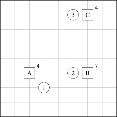
Figure 8.23 UFLP instance for Problem 8.20. Distances use Manhattan metric.
- The values of
- 8.21 (DUALOC #2) Repeat Problem 8.20 for the instance depicted
in Figure 8.24.

Figure 8.24 UFLP instance for Problem 8.21. Distances use Manhattan metric.
- 8.22 (Warehouses for Quikflix) Quikflix is a mail‐order DVD‐rental company. You choose which DVDs to rent on Quikflix's web site, and the company mails the DVDs to you. When you've finished watching the movies, you mail them back to Quikflix. Quikflix's business plan depends on fast shipping times (otherwise, customers will get impatient). But overnight delivery services like FedEx are prohibitively expensive. Instead, Quikflix has decided to open enough DCs so that roughly 90% of their customers enjoy 1‐day delivery times.
In this problem, you will formulate and solve a model to determine where Quikflix should locate DCs to ensure that a desired percentage of the US population is within a 1‐day mailing range while minimizing the fixed cost to open the DCs. (You may assume that the per‐unit cost of processing and shipping DVDs is the same at every DC.)
- Formulate the following problem as an integer programming problem: We are given a set of cities, as well as the population of each city and the fixed cost to open a DC in that city. The objective is to decide in which cities to locate DCs in order to minimize the total fixed cost while also ensuring that at least
 fraction of the population is within a 1‐day mailing range.
Define your notation clearly and indicate which items are parameters (inputs) and which are decision variables. Explain each of your constraints in words.
- Implement your model using a modeling language of your choice. Solve the problem using the data set provided in
quikflix.xlsx, which gives the locations and populations of the 250 largest cities in the United States (according to the 2000 US Census), as well as the average annual fixed costs to open a DC in the cities (which are fictitious). The file also contains the distance between each pair of cities in the data set, in miles. Assume that two cities are within a 1‐day mailing radius if they are no more than 150 miles apart.Using these data and a coverage percentage of
 , find the optimal solution to the Quikflix DC location problem. Include a printout of your model file (data not necessary) in your report. Report the total cost of your solution and the total number of DCs open.
- Formulate the following problem as an integer programming problem: We are given a set of cities, as well as the population of each city and the fixed cost to open a DC in that city. The objective is to decide in which cities to locate DCs in order to minimize the total fixed cost while also ensuring that at least
- 8.23 (Solving the Quikflix Problem) In Problem 8.22, you formulated an IP model to solve Quikflix's problem of locating DCs to ensure that a given fraction (
 ) of the population is within a 1‐day mailing range of its nearest DC. In this problem, you will develop a method for solving this IP using Lagrangian relaxation.
The IP formulation for Problem 8.22 contains two sets of decision variables. We'll assume that the x variables represent location decisions, while the z variables indicate whether or not a city is covered (i.e., is within a 1‐day mailing radius of an open facility). If you defined z as a continuous variable, make sure you have added a constraint requiring it to be less than or equal to 1. (This constraint is not strictly necessary since it is implied by other constraints, but it strengthens the Lagrangian relaxation formulation.)
The IP formulation also has a set of constraints that allow city i to be covered only if there is an open facility that is less than 150 miles away. If necessary, rewrite your model so that those constraints are written as
 constraints. Then relax those constraints, and let
  be the Lagrange multiplier for the constraint corresponding to node
  , where J is the set of cities.
- Write out the Lagrangian subproblem that results from this relaxation.
- The subproblem should decompose into two separate problems, one containing only the x variables and one containing only the z variables. Write out these two separate problems.
- Explain how to solve each of the two subproblems, the x‐subproblem and the z‐subproblem. Your solution method may not rely on using the simplex method or any other general‐purpose LP or IP algorithm.
- Suppose that the problem parameters and Lagrange multipliers are given by the following values:
i 


1 100 80 
2 100 120 
3 100 40 
4 100 90 
Suppose also that
 and that node 1 covers nodes 1, 2, 3; node 2 covers nodes 1, 2, and 4; node 3 covers nodes 1 and 3; and node 4 covers nodes 2 and 4.
Determine the optimal values of x and z, as well as the optimal objective value, for this iteration of the Lagrangian subproblem.
- 8.24 (UFLP with Enemy Customers) Suppose that, in the UFLP model, some pairs of customers are “enemies” and cannot be served by the same facility. Let
 if customers
  (
( ) are enemies of each other, 0 otherwise. (
 is a parameter.) Assume that the enemy pairs don't overlap: If i and k are enemies of each other, then i and k aren't enemies of any other customers.
- Write one or more linear constraints that can be added to the UFLP to enforce the condition that two customers may not be assigned to the same facility if they are enemies of each other. If you introduce any new notation, define it clearly.
- Suppose we add your constraints from part (a) to the UFLP and then relax constraints 8.4 using Lagrangian relaxation, with Lagrange multipliers
 . Write the resulting Lagrangian
subproblem.
. Write the resulting Lagrangian
subproblem. - Explain how to solve the Lagrangian subproblem you formulated in part (b) for fixed values of
 . Your solution method may not rely on using the simplex method or any other general‐purpose LP or IP algorithm.
 - Choose one option and briefly explain your reasoning: For every instance of the UFLP with enemy constraints, the optimal objective function value will be [
 ,
,  ,
,  ,
,  ,
,  ] the optimal objective function value of the corresponding instance of the classical UFLP.
 - Choose one option and briefly explain your reasoning: For every instance of the UFLP with enemy constraints, the optimal number of open facilities will be [
 ,
,  ,
,  ,
,  ,
,  ] the optimal number of open facilities in the corresponding instance of the classical UFLP.
- 8.25 (Locating Warehouses for Vandelay Industries) Vandelay Industries manufactures latex products at several plants (whose locations must be chosen from among a set of potential locations) and ships products to customers (whose locations and demands are known). There is a fixed cost to open each plant, and each has a fixed production capacity.
For each unit of demand shipped to a given customer, Vandelay Industries earns a certain amount of revenue. However, the company may choose to satisfy only a part of a given customer's demand, or not to satisfy its demand at all (for example, if it is too expensive to ship to that customer). The only penalty for failing to serve a customer is the lost revenue.
In order to ensure adequate service to customers spread throughout the country, Vandelay Industries also wishes to ensure that no two plants are located less than a certain distance apart.
The company's objective is to maximize the total profit, accounting for the revenue from serving customers and the costs of opening facilities and shipping goods to customers.
Formulate this problem as a linear mixed‐integer optimization problem (MIP). In addition to the notation in Sections 8.2.2 and 8.3.1, please use the following notation. If you use any additional notation, define it clearly.

= distance (miles) between plant  and plant

= minimum allowable distance (miles) between two open plants - 8.26 (Locating Snack Bars) You have been hired as a consultant for a new theme park to help choose locations for the park's snack bars (restaurants). The park has been divided into sectors, each representing a small area of land. The management team has forecast the number of people that are expected to be in each sector at any point in time.
Let I be the set of sectors and let J be the set of possible locations for the snack bars. The set J is a subset of I because each possible snack bar location is also a sector. Let
 be the number of people located in sector i, for
  . (Of course,
  is just an estimate, because this number will constantly be changing, but we'll treat it as though the number of people in sector i is static and deterministic.) Let
  be the number of minutes it takes to walk from sector i to sector j.
The management team has decided there will be four snack bars in the theme park. The snack bars are to be located so as to maximize the number of people that are within a 5‐minute walk of a snack bar. Let
 equal 1 if sector j is within a 5‐minute walk of sector i; that is,
Let
 equal 1 if we locate a snack bar in sector j and 0 otherwise (
 ). Let
  equal 1 if sector i is within a 5‐minute walk of a snack bar (
 ).
).- Formulate this problem as a linear mixed‐integer optimization problem (MIP). If you use any new notation, define it clearly. Explain your constraints in words.
- Suppose that the management team wants instead to maximize the number of customers covered by at least two snack bars. We can redefine
 to equal 1 if sector i is covered by at least two open snack bars. Explain how to modify your model from part (a) to enforce this new requirement. Clearly define any new notation you introduce and explain your new constraint(s) in words.
 - Return to the original formulation—assume again that a customer is “covered” if there is one open snack bar within 5 minutes. Suppose now the management team also wants to ensure that the average distance traveled by a customer to his or her closest snack bar is no more than 6 minutes. (The average is taken across all customers.) That is, we want to maximize the number of customers within 5 minutes of a snack bar, but we also want to ensure that the average time for all customers is no more than 6 minutes. Revise the model to include this requirement. Clearly define any new notation you introduce and explain any new constraints in words.
- Continuing with the model in part (c), suppose that the management wants to require that the average distance traveled by a customer to his or her second‐closest snack bar is no more than 6 minutes. Explain how to modify your model from part (c) to include this requirement. Clearly define any new notation you introduce and explain any new constraints in words.
- 8.27 (Locating RFID Readers) The theme park from Problem 8.26 issues bands to all of the visitors to the park. The bands are worn on the wrist, and they contain RFID chips that allow the park to identify visitors, without paper tickets, barcodes, etc. The RFID chips are “read” by RFID readers that are located throughout the park—at the park entrance, near the entrances to rides, and so on. RFID is wireless, and each RFID reader can detect RFID chips that are within a certain radius. In fact, there are two types of RFID readers—short‐range and long‐range—and the wrist bands contain both types of RFID chips. Some locations within the park must be covered by a short‐range reader, some by a long‐range reader, and some by both.
Two technical constraints restrict the locations of the readers:
- Short‐ and long‐range readers cannot be placed at the same location.
- No location can be covered by more than four readers, total (including both types).
Park planners want to locate RFID readers throughout the park to cover all of the necessary sites with the reader types required, at minimum possible cost, while satisfying the technical constraints.
- Let I be a set of nodes representing locations in the park that must be covered by an RFID reader. (We'll call these “demand nodes.”) Let J be a set of nodes representing potential sites for the readers. Let
 be the two types of readers (1 = short‐range, 2 = long‐range). Let
  be a parameter (an input) that equals 1 if demand node
  must be covered by a reader of type k. Let
  be the fixed cost to locate a type‐k reader at location
  . Let
. Let  be a decision variable that equals 1 if we locate a reader of type k at location
  .
.Using this notation, formulate the problem as a linear integer optimization model. Explain the objective function and the constraints in words. If you introduce any new notation, define it clearly.
- Now suppose the theme park's engineers have found a way to locate a short‐range and a long‐range RFID reader in the same location
 , but due to the expense involved in doing so, planners wish to have at most two locations that have both types of readers. Write one or more linear constraints to enforce this restriction.
- 8.28 (Locating Compost Sites) The city of Greentown is planning to open several composting facilities, which will convert organic matter (kitchen waste, leaves, yard waste, shredded paper, etc.) into fertilizer instead of sending it to landfills. While the population of Greentown agrees that this is a good idea, nobody wants a new compost site too close to their homes, due to the noise, smell, and truck traffic to and from the site. The city's mayor has hired you to develop a model to choose locations for the new compost facilities.
The population of the city has been aggregated into a set I of neighborhoods, each with population
 . City planners have identified a set J of potential sites for the compost facilities. The distance between neighborhood i and site j is given by
  miles. The city wishes to locate p compost sites in order to maximize the minimum distance between a neighborhood and its nearest open compost facility.
Define the following decision variables:

- Formulate this problem as a linear integer optimization model. Explain the objective function and constraints in words as well as formulating them in mathematical notation. If you introduce any new notation (sets, parameters, decision variables), define it clearly.
- Now suppose that, instead of maximizing the minimum distance between a neighborhood and its nearest open facility, the mayor wants to maximize the shortest distance between any two open compost facilities. Note that this objective function focuses only on the distances among compost facilities and ignores distances between facilities and neighborhoods.
Formulate this modified problem as a linear integer optimization model. Explain the objective function and new constraints in words. If you introduce any new notation, define it clearly.
- 8.29 (Convex Hulls are Nonoverlapping) Consider a facility location instance with nodes in
 and Euclidean distances. Suppose we open a set
  of facilities and assign each customer in I to the nearest open facility. Recall that the neighborhood of an open facility j is
  . Prove that the convex hulls
of the neighborhoods of the open facilities do not overlap.
. Prove that the convex hulls
of the neighborhoods of the open facilities do not overlap. - 8.30 (LR Iteration for UFLP) The
file
LR‐UFLP.xlsxcontains data for a 50‐node instance of the UFLP, as well as the Lagrange multipliers for a single iteration of the Lagrangian relaxation algorithm described in Section 8.2.3. For each facility , column
 Blists the fixed cost . For each customer
  , row
, row 2lists the demand and row
 3lists the Lagrange multiplier . Finally, the cells in the range
 C6:AZ55contain the matrix of transportation costs .
.- For each
 , calculate the benefit
  , the optimal value of
  , and the optimal objective value of
  . The worksheet labeled “
solution” contains spaces to list (column
 B), (column
 C), and the objective value (cellC5).Hint: To double‐check your calculations, we'll tell you that if
 and
and  , then
  .
. - Using the method described in Section 8.2.3.4, generate a feasible solution to the UFLP. In row
2of the “solution” worksheet, list the index of the facility that each customer is assigned to in your solution. In cellC6, list the objective value of your solution.
- For each
- 8.31 (Maxisum Location Problem) Consider the following problem: We must locate exactly p facilities, for fixed p. The objective is to maximize the sum of the demand‐weighted distances between each customer and its nearest facility. Formulate this problem as an IP. Define any new notation clearly. Explain the objective function and each of the constraints in words.
- 8.32 (Supplier–Facility Capacities) Consider the following extension of the UFLP: We are given a set K of suppliers whose locations are fixed. Each supplier
 can ship at most
  units to facility
  . This is like a capacity constraint, but it is (supplier, facility)‐specific rather than the facility‐specific capacities discussed in Section 8.3.1. Such constraints might arise from, say, the capacity of the truck transporting goods from k to j. Let
  be the cost to transport one unit of demand from supplier
  to facility
  , and let
  be a decision variable representing the number of units transported from k to j. Note that
  is a flow‐type variable (
 ), whereas
  is a fractional variable (
 ). Multiple‐sourcing is allowed; that is, facility j may receive shipments from more than one supplier k. In addition to the notation just defined, use the notation in Section 8.2.2. If you need to define any additional notation, define it clearly.
- Formulate this extension of the UFLP as a linear mixed‐integer optimization problem. Explain the objective function and each constraint clearly in words.
- In Section 8.2.3, we solved the UFLP by relaxing the “assignment” constraints that require each customer to be assigned to exactly 1 facility. Write the objective function of the Lagrangian subproblem that results from relaxing the analogous constraint in your model from part (a).
- Consider the special case in which
 for all
  , i.e., all of the customers have the same demand, and
  is an integer multiple of h for all j, k. Explain how to solve the Lagrangian subproblem from part (b) for this special case. Your method must be exact (i.e., it must be guaranteed to find the optimal solution) and self‐contained (i.e., it may not rely on a general‐purpose optimization solver).
 - Describe a method that, given a feasible solution to the Lagrangian subproblem, produces a feasible solution for the original problem.
- 8.33 (Salt Stockpiles) You are the director of your local Department of Transportation. You have decided to build silos to stockpile the salt the department uses on roadways during winter weather. A stockpile is considered to cover a town if they are within r miles of each other. Your job is to determine where to locate up to p stockpiles to maximize the total population of the towns that are double‐covered, i.e., covered by at least two stockpiles. Local planners have provided you with the population of each town that you would like to be covered.
- Formulate this problem as an integer programming problem. Define any new notation clearly.
- Now suppose that the two stockpiles that double‐cover a given town must be at least s miles from each other. (Two stockpiles may be located less than s miles from each other, but a given town doesn't count as double‐covered unless there are two stockpiles that cover it and that are at least s miles apart.) Formulate the new model, and define any new notation clearly.
- 8.34 (Pre‐Positioning Disaster Relief Shelters) A
disaster relief agency plans to establish shelters in preparation for a hurricane that has been forecast for the coming days. The agency wishes to choose shelters from a set J of potential locations in order to cover every population center in the set I. A shelter covers a population center if it is within r miles of it. As in the set covering and maximal covering models, we define the parameter
 to equal 1 if a shelter at site
  covers population center
  .
.If we locate a shelter at site j, we incur a fixed cost of
 , as well as an “assignment cost” of
  for each population center assigned to the shelter at j (regardless of the size of these population centers). For example, if shelter j serves 12 population centers, then we pay an assignment cost of
  .
.Define the following decision variables:

- Formulate this problem as a linear integer optimization problem. If you introduce any new notation, define it clearly. Briefly explain your objective function and constraints.
- In part (a), the assignment cost is a linear function of the number of population centers assigned to each shelter: It equals
 , where n is the number of population centers assigned to j. Suppose instead that the assignment cost is a nonlinear function
  , where n is the number of population centers assigned to j. Define the following decision variables:Formulate this problem as a linear integer programming problem. Define any new notation clearly, and explain the objective function and any new constraints.
- 8.35 (Stochastic Pre‐Positioning) A humanitarian relief agency wishes to pre‐position stockpiles of emergency supplies (food, water, blankets, medicine, etc.) for use in the aftermath of disasters. Its objective is to locate the smallest possible number of stockpiles while ensuring a low probability that, for each population center, a disaster strikes and the population center cannot be served by any stockpile. Whether a given stockpile can serve a given population center depends on their physical distance as well as on the disaster that strikes.
Disasters are represented by scenarios. A scenario can be thought of as a disaster type, magnitude, and location (e.g., magnitude 7.5 earthquake in city A, influenza pandemic in city B, etc.). However, mathematically each scenario simply specifies whether a given population center can be served by a given stockpile during a given disaster.
Let I be the set of population centers, and let J be the set of potential stockpile locations. Let S be the set of scenarios (including the scenario in which no disaster occurs), and let
 be the probability that scenario s occurs. Stockpile j is said to “cover” population center i in scenario s if either stockpile j can serve population center i in scenario s or population center i does not need disaster relief in scenario s. Let
  be a parameter that equals 1 if stockpile j covers population center i in scenario s, and 0 otherwise. Assume each stockpile is sufficiently large to serve the needs of the entire population it covers.
Formulate a linear integer programming problem that chooses where to locate stockpiles in order to minimize the total number of stockpiles located while ensuring that, for each
 , the probability that i is not covered by any open stockpile is less than or equal to
  , for given
  . Clearly define any new notation you introduce. Explain the objective function and all constraints
in words.
. Clearly define any new notation you introduce. Explain the objective function and all constraints
in words. - 8.36 (Error Bias) Suppose the transportation costs are estimated badly in the UFLP. It is natural to expect that the true cost of the solution found under the erroneous data has an equal probability of being larger or smaller than the cost calculated when solving the problem. Test this hypothesis by solving the instance given in
random‐errors.xlsx100 times, each time perturbing the transportation costs by multiplying them by random variates. For each instance generated this way, record the objective function value, as well as the objective function of the same solution when the correct costs are used. If the hypothesis is correct, the objective function should be less than the true cost for roughly half of the instances and greater for the other half. Do your results confirm the hypothesis? In a few sentences, explain your results, and why they occurred. Also comment on the implications your results have for the importance of having accurate data when choosing facility
locations.
random variates. For each instance generated this way, record the objective function value, as well as the objective function of the same solution when the correct costs are used. If the hypothesis is correct, the objective function should be less than the true cost for roughly half of the instances and greater for the other half. Do your results confirm the hypothesis? In a few sentences, explain your results, and why they occurred. Also comment on the implications your results have for the importance of having accurate data when choosing facility
locations. - 8.37 (1‐Center on a Tree) Consider the 1‐center problem on a tree network in which all of the demands are 1. Prove that the Algorithm 8.10 finds the optimal solution to both the absolute
and the vertex 1‐center problem.
(Recall from Section 8.4.3 that the absolute p‐center problem allows facilities to be located on either the edges or the nodes of the network, whereas the vertex p‐center problem restricts facilities to the nodes.)

- 8.38 (2‐Center on a Tree) Prove that Algorithm 8.11 finds the optimal solution to the absolute 2‐center problem.
- 8.39 (N‐Echelon Location Problem)
By extending the approach used in Section 8.7.1, formulate a facility location model with N echelons, for general
 . Echelon N ships products to echelon
  , which ships products to echelon
  , and so on; echelon 1 serves the end customer. The locations of the facilities in echelons
  are to be decided by the model, and there are fixed costs for each. Define any new notation clearly. Explain the objective function and each of the constraints in words. Note: No decision variables should have more than 3 indices.

- 8.40 (UFLP Duality Gap) Prove Lemma 8.4.
- 8.41 (Another Relaxation for the pMP) Suppose that we use Lagrangian relaxation to relax constraint 8.72 in the pMP. Write the resulting Lagrangian subproblem. This problem is structurally identical to another problem discussed in this chapter; what is it? Briefly summarize the advantages and disadvantages of this relaxation compared to the relaxation discussed in Section 8.3.2.2: Which subproblem is harder to solve? Which approach will give a tighter bound? For which approach will the subgradient optimization procedure converge more quickly?
- 8.42 (Tightening the CFLP Relaxation) Suppose
we add the following constraint to the CFLP:
Explain in words what this constraint says. Explain why this constraint is redundant for the CFLP (adding it does not change the optimal solution for the CFLP) and why adding it tightens the Lagrangian relaxation discussed in Section 8.3.1. Finally, explain how to solve the Lagrangian subproblem when constraint 8.152 is included in the model.
- 8.43 (Variable‐Splitting Method for CFLP) In
this problem, you will develop a variable‐splitting method for the CFLP. Variable splitting (also known as Lagrangian decomposition) is a method that involves duplicating one or more sets of variables, adding a constraint that requires those variables to be equal to their duplicates, and then relaxing that constraint using Lagrangian relaxation. (See Guignard and Kim (1987).)
- Introduce new decision variables
 for
for  ,
,  . Rewrite the objective function aswhere
 is a constant. Rewrite constraints 8.55 using w instead of y. Add the following new constraints, which require w and y to be equal, and require w to be nonnegative:
(8.154)Write the resulting problem. This problem is equivalent to (CFLP).
is a constant. Rewrite constraints 8.55 using w instead of y. Add the following new constraints, which require w and y to be equal, and require w to be nonnegative:
(8.154)Write the resulting problem. This problem is equivalent to (CFLP).
- Relax constraints 8.153 using Lagrangian relaxation. Write the resulting subproblem.
- Explain how to solve the subproblem from part (b).
- Based on your intuition, will this relaxation provide a tighter, weaker, or equivalent bound to the relaxation discussed in Section 8.3.1?
- Introduce new decision variables
- 8.44 (Accuracy of Spherical Law of Cosines Formula)Calculate
the distances between every pair of nodes in the 88‐node data set (
88node.xlsx) using both the great circle distance formula 8.1 and the spherical law of cosines formula 8.2. Compare the results. Are there any cases for which the two formulas produce distances that differ by more than a mile or so? If so, what characterizes those cases? - 8.45 (Swap vs. Neighborhood Search for p‐Median) Implement the swap and neighborhood search heuristics for the pMP (Algorithms 8.7 and 8.8). Conduct a numerical experiment to compare the effectiveness (as measured by objective function value) and efficiency (as measured by CPU time) of these two heuristics. Your experiment should use randomly generated p‐median instances with at least 100 nodes.
- 8.46 (Hakimi Property for SCLP) Does the Hakimi property hold for the set covering problem? Explain your answer.
- 8.47 (Proof of Lemma 8.8) Prove Lemma 8.8.
- 8.48 (Solving the pCP using the MCLP) Algorithm 8.9 relies
on the relationship between the pCP and the SCLP stated in Lemma 8.8. A similar relationship exists between the pCP and the MCLP.
- State a lemma similar to Lemma 8.8 that describes this relationship.
- Write pseudocode similar to Algorithm 8.9 for an exact algorithm that solves the pCP by iteratively solving MCLPs.
- 8.49 (The MCLP with Mandatory Closeness Constraints) The
MCLP with mandatory closeness constraints is identical to the MCLP except that it also requires every customer to be covered within a distance of s, with
 . That is, we wish to maximize the number of demands that are covered within r, but every customer must be covered within s. Write an integer programming formulation for this problem. If you introduce any new notation, define it clearly. Explain the objective function and each constraint in words.
 - 8.50 (MCLP is a Special Case of pMP) Show that the MCLP is a special case of the pMP by showing how to set the parameters of the pMP so that solving it is equivalent to solving the MCLP.
- 8.51 (A Dynamic Location Problem) Consider a dynamic facility location problem in which the demands over a finite time horizon are known but change in each time period:
 is the demand at node
  in period t, where
  . We can open and close as many facilities as we like in each time period. Facility
  incurs a fixed cost of
  if it is opened in period t (but was closed in period
  ), a fixed cost of
  if it is closed in period t (but was open in period
  ), and a fixed cost of
  if it remains open in period t (that is, if it was also open in period
  ). Assume that no facilities are open at the start of the horizon, that is, in period 0. The transportation cost from facility j to customer i in period t is given by
  . Formulate an integer programming model to optimize the locations of facilities over the time horizon to minimize the total fixed and transportation costs. If you introduce any new notation, define it clearly. Explain your objective function and constraints in words.
 - 8.52 (MCLP Modifications) Modify the MCLP to accommodate each of the changes described below (one at a time). For each modification, change either the objective function or exactly one constraint to reflect the modification. Indicate the number of the equation (objective function or constraint) you are changing.
- We wish to maximize the total number of nodes covered, not the total population covered.
- Each facility j has a fixed construction cost of
 . Rather than restricting the number of facilities to equal p, restrict the total amount spent to construct facilities to a budget of b.
 - A demand node only counts as covered if there are two facilities within the coverage radius.
- 8.53 (Subproblem Assignments) Prove that, if customer i is assigned to at least one facility in the optimal solution to (UFLP‐LRλ), then one of the facilities it is assigned to is the nearest open facility. (This implies that in step 4 of Algorithm 8.2, it suffices to check only those j such that
 in the optimal solution to (UFLP‐LRλ).)
 - 8.54 (Location of Power Generators) Consider
the problem of locating generators within an electricity network.
- First consider a single generator. Suppose the generator's load (i.e., the total demand for electricity from the generator) is given by
 , where D is measured in kilowatt‐hours (kWh). The cost to generate enough electricity to meet a load of d kWh is given by
  , where
  is a constant. Prove that the expected generation cost is given by
  .
. - Now consider an electricity network consisting of multiple generators, whose locations we need to choose. Let I be the set of loads (demand nodes), with load i having a daily demand distributed
 . Let J be the set of potential generators. The daily fixed cost if generator j is open is
  , and the generation cost coefficient for j is
  . Formulate the problem of choosing generator locations and assigning loads to generators in order to minimize the expected daily cost of the system. Assume that, once location and assignment decisions are made, the power network for a given generator and its loads is disconnected from the remaining generators and loads (so that the physics of power flows can be ignored). Also assume that the cost to transmit power is negligible.
- First consider a single generator. Suppose the generator's load (i.e., the total demand for electricity from the generator) is given by
- 8.55 (Stochastic Location for Toy Stores) Return to Problem 8.1, and suppose now that the demands are stochastic. The file
toy‐stores‐stochastic.xlsxgives the demands for five scenarios, as well as the probability that each scenario occurs.- Implement the stochastic fixed‐charge location problem in a modeling language of your choice. Find the optimal solution for the instance given in the data set. Report the optimal set of facilities and the corresponding cost.
- Now implement and solve the minimax fixed‐charge location problem. Report the optimal set of facilities and the corresponding cost.
- 8.56 (Minimax Cost
 Minimax Regret) Construct
a small example of the minimax fixed‐charge location problem (MFLP) in which minimizing the maximum cost results in an optimal solution that is different from the solution that minimizes the maximum regret. (You may choose either relative or absolute regret.) Your instance may have at most five nodes.
Minimax Regret) Construct
a small example of the minimax fixed‐charge location problem (MFLP) in which minimizing the maximum cost results in an optimal solution that is different from the solution that minimizes the maximum regret. (You may choose either relative or absolute regret.) Your instance may have at most five nodes. - 8.57 (Side Constraints for Arc Design) Formulate each side constraint listed below for the arc design model in Section 8.7.2.2. Your constraints must be linear. If you introduce any new notation, define it clearly.
- We have a set
 of ordered pairs of arcs such that, for
  , if arc
  is opened, then arc
  must be opened.
 - We have a set of
 of arcs such that at most r arcs in
  may be opened.
 - We have a set of
 of arcs such that at least r arcs in
  must be opened.
 - We have an upper bound B on the transportation cost that may be spent shipping on a subset
 of the arcs.
- We have a set
- 8.58 (Modified Hungary Network) Consider the Hungary instance of the arc design problem shown in Figure 8.20. The file
hungary2.xlsxcontains a modification of the instance described in Example 8.11. It lists the latitude and longitude of each node, the available units for each node and product, and the fixed cost and capacity for each arc. The variable cost is 1 for every arc and product. Formulate the arc design model in a modeling language of your choice, and solve this instance. Report the optimal arcs to open, the optimal flows, and the optimal total cost. - 8.59 (Campaign Offices) A candidate for a national political position wishes to establish campaign offices and decide how much money to spend on campaign activities at those offices. The candidate's staff has identified a set J of potential locations for campaign offices (facilities) and a set I of neighborhoods (demand nodes) that they wish to “cover” using these offices. Let
 be a parameter that equals 1 if office location
  covers neighborhood
  , and 0 otherwise. Neighborhood
  has
has  registered voters living in it. Opening an office at location
  incurs a fixed cost of
  .
.In addition to choosing where to locate offices, the candidate's staff needs to determine how much money to spend on campaign activities (get‐out‐the‐vote, marketing, etc.) at each office. They can only perform campaign activities at offices that they have chosen to open. Staffers have estimated that each $1 spent on these activities will earn the candidate exactly one extra vote.
For example: Suppose the candidate opens an office at location
 , and location j covers 1000 registered voters. If the campaign spends $1000 on campaign activities (not including the fixed cost
  ), the candidate will earn all of their votes; if it spends $500, the candidate will earn half of their votes; and if it spends $0, the candidate will earn none of their votes. Note that there is no advantage to spending more than $1000 on campaign activities in this example. There is also no advantage to opening an office at j if we spend $0 since the candidate will not earn any votes.
If a neighborhood is covered by more than one open campaign office, its votes can only be earned once. Therefore, only one office should direct its campaign activities at that neighborhood. Your model should choose which of the open offices should “serve” each customer.
The candidate's objective is to maximize the number of votes earned. The campaign has a total budget of $B to spend on both fixed costs and campaign activities.
Define the following decision variables:

= 1, if we open a campaign office at location  , 0 otherwise
= the number of dollars we spend on campaign activities at office 
Formulate this problem as an integer linear optimization problem. If you introduce any new notation, define it clearly. Explain your objective function and each constraint in words.
- 8.60 (Exchange Rate Hedging) An automobile manufacturer wishes to decide where to locate factories around the world in order to account for random fluctuations in currency exchange rates. The company will change the production levels at the various factories to take advantage of changes in the exchange rates. Exchange rates are expressed as
 $/¤, where $ stands for US dollars (USD) and ¤ stands for the local currency in the other country. For example, if the exchange rate between the United States and Thailand is
  $/???, then 1 Thai baht is worth US$0.028.
The manufacturer is considering a set J of potential locations for the factories, which will ship automobiles directly to the customers in a set I. Customer
 has a demand of
  units per year. We have the following costs:
- Building a factory at site
 incurs a fixed annual cost of $
 , which is deterministic and expressed in USD.
 - The cost to produce one automobile at factory
 is ¤
is ¤ , which is deterministic and expressed in the local currency of the country in which factory j is located.
 - The cost to ship one automobile from factory
 to customer
  is $
is $ , which is deterministic and expressed in USD.
The factories have effectively unlimited capacity.
Once the factories are built, the random exchange rates are realized, and the company then decides how much to produce at each factory, as well as how much to ship from each factory to each customer. The exchange rates are described by a set S of scenarios, such that
 is the exchange rate (in $/¤) in scenario s for the country in which facility
  is located. Let
  be the probability that scenario s occurs.
Let
 equal 1 if we open a factory at site
  , 0 otherwise. Let
  equal the number of automobiles to be shipped from a factory at site
  to customer
  in scenario
  . These are our decision variables. You may treat
  as a continuous variable.
- Formulate a stochastic optimization problem that minimizes the total expected annual cost of locating facilities and producing and transporting automobiles. If you introduce any new notation, define it clearly. Explain your objective function and each constraint in words.
- Suppose we allow
 to be continuous and nonnegative. If the demands
  are expressed as integers, will there necessarily exist an optimal solution in which the
  are integers? Why or why not?
 - Suppose that, instead of minimizing the total expected cost, the company wishes to minimize the maximum absolute regret that can occur, across all exchange rate scenarios. Formulate this new problem. If you introduce any new notation, define it clearly.
- Building a factory at site