
Chapter 7
Pooling and Flexibility
7.1 Introduction
The stochastic inventory models in Chapters 4–6 assume that inventory is the only tool for mitigating uncertainty. In contrast, this chapter examines uncertainty mitigation using other means. In all of the strategies covered here, the idea is to “pool” multiple demand streams in some way, and to share some resource—inventory or capacity—among them. Because not all of the demand streams will need all of the resources at all times, there is no need to dedicate whole resources to each stream. By pooling them, we can reduce the amount of safety stock required to meet a given service level (or increase the service level attained by a given level of safety stock).
Section 7.2 deals with risk pooling, in which we physically combine the inventories used to satisfy multiple demand streams, by storing them together in the same warehouse. Section 7.3 discusses a strategy called postponement, in which we differentiate products later in their manufacturing process. This allows a reduction in inventory since multiple demand streams (from different end products) are sharing inventory of the the undifferentiated product. The cost savings from postponement is due to the risk pooling effect.
Another way that inventory can be pooled is by allowing transshipments—“lateral” transfers of inventory from one retailer to another when one has extra inventory and the other has a shortage. In Section 7.4, we discuss a model for deciding how much inventory to hold at a given retailer, anticipating that transshipments either to or from that retailer may occur later in the period. The benefit from transshipments is similar to that from risk pooling, although there is no physical pooling of inventory.
Similarly, when multiple products are sold, and each product is manufactured by a dedicated plant, it is sometimes beneficial for one plant to make multiple products so that when one product has very high demand (exceeding the capacity of a plant that makes the product), other plants can help produce more units of the product to meet the demand. In this case, we have “lateral” transfers of production capacity, in a strategy known as process flexibility. We can think of process flexibility as a type of pooling that occurs when the product is manufactured, rather than when it is stored. We discuss process flexibility in Section 7.5.
7.2 The Risk‐Pooling Effect
7.2.1 Overview
Consider a network consisting of N distribution centers (DCs)
or other facilities, each of which faces random demand
for a single product. The DCs each hold inventory of this product. In fact, they act like N independent newsvendors, each facing ![]() demand per period. If the DCs each wish to meet a type‐1 service level
of
demand per period. If the DCs each wish to meet a type‐1 service level
of ![]() (that is, they wish to stock out in no more than
(that is, they wish to stock out in no more than ![]() % of the periods on average), they must each hold an amount of safety stock
equal to
% of the periods on average), they must each hold an amount of safety stock
equal to ![]() (from (4.24)). The total safety stock in this system is therefore
(from (4.24)). The total safety stock in this system is therefore ![]() . (See Figure 7.1(a).)
. (See Figure 7.1(a).)
Now suppose that all N DCs are merged into a single DC. What are the inventory implications of this consolidation? (We're ignoring the possible increase in transportation cost, lead time, and hassle the consolidation may cause.) The new DC's demand process is equal to the sum of all of the original DCs' demands. This process has a mean demand of ![]() and a standard deviation of
and a standard deviation of ![]() . Therefore, to meet the same service level (
. Therefore, to meet the same service level (![]() ), the new DC needs to hold
), the new DC needs to hold ![]() of safety stock (see Figure 7.1(b)), which is less than the safety stock required when N DCs each hold
inventory.
of safety stock (see Figure 7.1(b)), which is less than the safety stock required when N DCs each hold
inventory.

Figure 7.1 The risk‐pooling effect with identical retailers.
This phenomenon is known as the risk‐pooling effect (Eppen, 1979). The basic idea is that by pooling demand streams, we can reduce the amount of safety stock required to meet a given service level, and hence, we can reduce the holding cost.
We next discuss the risk‐pooling effect in greater generality. Our analysis is adapted from that of Eppen (1979).
7.2.2 Problem Statement
We'll assume that each DC follows a base‐stock inventory policy
under periodic review,
with ![]() the base‐stock level
for DC i. The lead time is
the base‐stock level
for DC i. The lead time is ![]() at every DC. Excess inventory may be stored from period to period (with a holding cost
of h per unit per period), and excess demand is backordered
(with a penalty cost of p per unit per period). We assume
at every DC. Excess inventory may be stored from period to period (with a holding cost
of h per unit per period), and excess demand is backordered
(with a penalty cost of p per unit per period). We assume ![]() . Note that h and p are the same at every DC.
. Note that h and p are the same at every DC.
The demand per period seen by DC i is represented by the random variable ![]() , with
, with ![]() .
Let
.
Let ![]() and
and ![]() be the pdf and cdf, respectively, of
be the pdf and cdf, respectively, of ![]() . Demands may be correlated among DCs.
The covariance of
. Demands may be correlated among DCs.
The covariance of ![]() and
and ![]() is given by
is given by ![]() and the correlation coefficient by
and the correlation coefficient by ![]() ; then
; then ![]() . (Corbett and Rajaram (2006) extend these results to general probability distributions and dependence structures.)
. (Corbett and Rajaram (2006) extend these results to general probability distributions and dependence structures.)
For each DC, the sequence of events in each period is the same as in Section 4.3.
7.2.3 Decentralized System
We will refer to the N‐DC system as the decentralized system since each DC operates independently of the others. ![]() is the base‐stock level
at DC i; this is a decision variable. The expected cost per period at DC i can be expressed as a function of
is the base‐stock level
at DC i; this is a decision variable. The expected cost per period at DC i can be expressed as a function of ![]() as follows:
as follows:
This formula is identical to the formula for the newsvendor cost (4.3) except for the subscripts i. Therefore, from Theorems 4.1 and 4.2, the optimal solution is
where ![]() and
and ![]() is the
is the ![]() th fractile of the standard normal distribution,
and the optimal cost at DC i is
th fractile of the standard normal distribution,
and the optimal cost at DC i is
(Recall that ![]() is the pdf of the standard normal distribution.) Defining
is the pdf of the standard normal distribution.) Defining ![]() for convenience, the optimal total expected cost (at all DCs) in the decentralized system, denoted
for convenience, the optimal total expected cost (at all DCs) in the decentralized system, denoted ![]() , is
, is

7.2.4 Centralized System
Now imagine that the DCs are consolidated into a single DC, denoted with index 0, that serves all of the demand. We will refer to this as the centralized system. Let ![]() be the total demand seen by this super‐DC. Its mean and standard deviation are
be the total demand seen by this super‐DC. Its mean and standard deviation are

(Note that by definition, ![]() .) Similar logic as above shows that the optimal base‐stock level for the centralized system is
.) Similar logic as above shows that the optimal base‐stock level for the centralized system is
with optimal expected cost

7.2.5 Comparison
Now let's compare the centralized and decentralized systems. The next theorem says that the centralized system is no more expensive than the decentralized system. This is the risk‐pooling effect.
One interpretation of the risk‐pooling effect is that pooling inventory allows the firm to take advantage of random fluctuations in demand. If one DC sees unusually high demand in a given time period, it's possible that another DC sees unusually low demand. In the centralized system, the excess inventory at the low‐demand DC can be used to make up the shortfall at the high‐demand DC. In the decentralized system, there is no opportunity for this supply–demand matching.
A more mathematical explanation is that risk pooling occurs because the centralized system takes advantage of the concave nature of safety stock requirements. The amount of safety stock required is proportional to the standard deviation of demand. The standard deviation of demand at the centralized site is smaller than the sum of the standard deviations of the individual sites in the decentralized system since variances, not standard deviations, are additive.
Somewhat surprisingly, the variances of the costs of the centralized and decentralized systems are equal at optimality; that is,
where

are the costs in the decentralized and centralized systems, respectively, for given (random) values of the demands.
7.2.6 Magnitude of Risk‐Pooling Effect
Let's try to get a handle on the magnitude of the risk‐pooling effect. Let

Note that

Uncorrelated Demands: First assume that the demands are uncorrelated, i.e., ![]() for all
for all ![]() , so
, so ![]() . Then
. Then

The magnitude of the difference between ![]() and
and ![]() depends on the magnitude between
depends on the magnitude between ![]() and
and ![]() .
.
Positively Correlated Demands: Next
suppose that demands are positively correlated. In fact, consider the extreme case in which ![]() for all
for all ![]() . Then
. Then

so there is no risk‐pooling effect at all (in the extreme case of perfect correlation).Negatively Correlated Demands: Finally,
assume that demands are negatively correlated. It's difficult to identify the extreme case since ![]() can't equal
can't equal ![]() for all
for all ![]() . (Why?) But we can say that
. (Why?) But we can say that ![]() since
since

So let's assume as an extreme scenario that ![]() . Then
. Then

The centralized cost is 0, while the decentralized cost is not.
So the risk‐pooling effect is very pronounced when demands are negatively correlated, smaller when demands are uncorrelated, and smaller still, or even non‐existent, when demands are positively correlated. Why? Recall the explanation given in Section 7.2.5: The risk‐pooling effect occurs because excess inventory at one DC can be used to meet excess demand at another. If demands are negatively correlated, there is a lot of opportunity to do this since demands will be very disparate at different locations. On the other hand, if demands are positively correlated, they tend to be all high or all low at the same time, so there is little opportunity for supply–demand rebalancing.
7.2.7 Closing Thoughts
The analysis above only considers holding and stockout costs ; it does not consider fixed costs (to build and operate DCs) or transportation costs. Clearly, as DCs are consolidated, the fixed cost will decrease. But the transportation cost will increase, since retailers (or other downstream facilities) will be served from more distant DCs. In many cases, the magnitude of the risk‐pooling effect may be far outweighed by the increases or decreases in fixed and transportation cost. Any analysis of a potential consolidation of DCs must include all factors, not just risk pooling. The location model with risk pooling (LMRP), discussed in Section 12.2, attempts to incorporate all of these factors when choosing facility locations.
7.3 Postponement
Many firms have product lines containing closely related products. In many cases, multiple end products are made from a single generic product. For example, the clothing retailer Benetton sells many colors of sweater, each of which comes from the same white sweater that's dyed multiple colors (Heskett and Signorelli, 1984). Hewlett‐Packard sells the same printer in dozens of countries, with a different power supply module, manual, and labels in each (Feitzinger and Lee, 1997; Lee and Billington, 1993). IBM builds individualized computers by building partially finished products called “vanilla boxes” and customizing them to order (Swaminathan and Tayur, 1998).
A key question in the design of the manufacturing process for each of these products is: When should the end products be differentiated? For example, consider a manufacturer of mobile phones that sells phones in many countries. The company programs each phone with a given language at the factory—the phone is “localized” when it is manufactured. The number of phones to be programmed in each language is determined based on a forecast of the demand in each country. The phones are then shipped to regional DCs, approximately one on each continent. The regional DCs store the phones until they are required by retailers, at which point they are shipped to individual countries. If the demand forecasts were wrong, and demand for phones in, say, Thailand was higher than expected while demand in Holland was lower than expected, the company would have to correct this discrepancy by reprogramming some of the Dutch phones into Thai phones, then shipping them from the Europe DC to the Asia DC—a costly and time‐consuming proposition.
Now suppose that generic phones are shipped to the regional DCs, and languages are programmed at the DCs once the phones are requested by retailers. Since the phones are localized on demand, there is much less risk of having too many phones of one language and too few of another. In addition, the firm holds inventory of generic phones, not localized phones, which means that fewer phones need to be held in safety stock due to the risk‐pooling effect, as we will see below.
This strategy is called postponement or delayed differentiation. The idea is to delay, as much as possible, the point in the manufacturing process at which end products are differentiated from one another. Of course, designing a postponement strategy may be extremely complicated, since it may require the redesign of the product and the manufacturing and distribution processes. In the mobile phone example, the regional DCs would have to be outfitted with language‐programming equipment.
To take the Benetton example to an extreme, postponement might mean that sweaters are dyed in the retail stores once they are demanded by a customer. You would request, say, a red sweater, and it would be dyed for you on demand; stores would never be out of stock of the sweater you wanted. This seems silly, since the costs of implementing such a system would probably far outweigh the benefits. But some products are actually sold this way. For example, paint is mixed to order from generic white paint at your hardware store, giving you access to an enormous range of colors that would be prohibitively expensive to keep in stock. (See Lee (1996) for a discussion of the benefits and challenges of postponement.)
The cost savings from postponement is due to the risk‐pooling effect: Generic products represent pooled inventory, while end products represent decentralized inventory. Suppose there are N end products. If the products are differentiated at the beginning of the manufacturing process (so that separate inventory is held of each end product), then the total safety stock required is

which is proportional to the safety stock required in the decentralized system in our discussion of risk pooling. Similarly, if the products are differentiated at the end (so that only a single inventory pile is required), the total safety stock is

which is proportional to the safety stock in the centralized system.
7.4 Transshipments
7.4.1 Introduction
When multiple retailers stock the same product, it is sometimes advantageous for one retailer to ship items to another if the former has a surplus and the latter has a shortage. Such “lateral” transfers are called transshipments. Transshipments are a mechanism for improving service levels since they allow demands to be satisfied in the current period when they might otherwise be lost or backordered until the following period. In that regard, the benefit from transshipments is very similar to that from risk pooling, since transshipments use one retailer's surplus to reduce another retailer's shortfall. In this case, however, there is no physical pooling of inventory, though the strategy is sometimes referred to as “information pooling.” Of course, transshipments come at a cost: Transshipments are often more expensive than replenishments from the DC because they are smaller and therefore lack the economies of scale from larger shipments.
In this section, we will discuss a model for setting base‐stock levels in a system with two retailers that may transship to one another. This model is adapted from Tagaras (1989). For models with more than two retailers, see Krishnan and Rao (1965), Tagaras (1999), or Herer et al. (2006).
This model will assume that transshipments occur after the demand has been realized but before it must be satisfied. Therefore, these transshipments are reactive since they are made in reaction to realized demands. In contrast, one might consider proactive transshipments that are made in anticipation of demand shortages. Proactive transshipments are of interest when demands must be met instantaneously, since there is no opportunity for transshipping between demand realization and satisfaction. On the other hand, proactive transshipments are more complex to model, so we will focus only on reactive transshipments. We will develop an analytical expression for the expected cost function, but the expected cost can only be minimized using numerical methods (rather than using differentiation). We will also discuss the improvement in service levels due to transshipments.
7.4.2 Problem Statement
Consider a system with two retailers served by a single DC. The retailers receive replenishment shipments from the DC and are permitted to transship goods to each other. As previously stated, transshipment occurs after the demand has been realized but before it must be satisfied. This is a periodic‐review
model with an infinite horizon.
There is no fixed cost and no lead time, either for replenishments or transshipments. Each retailer i (![]() ) follows a base‐stock policy,
with base‐stock level
) follows a base‐stock policy,
with base‐stock level ![]() .
The demand at retailer i is a random variable
.
The demand at retailer i is a random variable ![]() with pdf
with pdf ![]() and cdf
and cdf ![]() . If there are excess demands at a retailer after transshipments have been made, they are
backordered. The costs are as follows:
. If there are excess demands at a retailer after transshipments have been made, they are
backordered. The costs are as follows:
|
|
= ordering cost per unit at retailer i, for |
|
|
= holding cost per unit per period at retailer i, for |
|
|
= backorder cost per unit per period at retailer i, for |
|
|
= cost per unit to transship from i to j, for |
We will assume that
In other words, it is cheaper to ship directly to j than to ship to i and then transship to j. This is sometimes referred to as a triangle inequality. We will also make the following assumptions:
-
 (i.e., if there is a shortage at j and a surplus at i, it is better to transship than not to, since the cost to transship is
  , while the cost to do nothing is
  (since we would incur the holding cost at i, the penalty cost at j, and then next period we'd order one more unit at j and one fewer at i))
 -
 (i.e., don't transship if there is a surplus at both retailers)
 -
 (i.e., don't transship if there is a shortage at both retailers)
These three assumptions imply that complete pooling is optimal: Transship if one retailer has a surplus while the other has a shortage, but if both have surpluses or both have shortages don't transship—one retailer's demand is not “more valuable” than the other's.
The sequence of events in each period is as follows:
- Retailers observe their inventory levels.
- Each retailer i places a replenishment order of size
 to the DC and receives it instantaneously.
 - Demand is observed.
- Transshipment decisions are made. Transshipments are sent and arrive instantaneously.
- Demand is satisfied to the extent possible, and excess demands are backordered.
- Holding and stockout costs are assessed.
We will make use of the following random variables:
|
|
= replenishment order quantity at retailer i, for |
|
|
= amount transshipped from i to j, for |
|
|
= inventory level at retailer i after step 5, for |
|
|
= on‐hand inventory at retailer i after step 5, for |
|
|
= backorders at retailer i after step 5, for |
Then
Note that these are all random variables—they are not decision variables. The decision variables are ![]() , the base‐stock levels for
, the base‐stock levels for ![]() . We will compute expectations of the random variables once the base‐stock levels are set, in order to compute the expected cost.
. We will compute expectations of the random variables once the base‐stock levels are set, in order to compute the expected cost.

Figure 7.2 Possible realizations of transshipment and ending inventories..
Adapted with permission from Tagaras, Effects of pooling on the optimization and service levels of two‐location inventory systems, IIE Transactions, 21, 1989, 250–257. ©1989, Taylor & Francis, Ltd.,
http://www.informaworld.com
The complete pooling policy can be stated formally as follows:
- If
 for
for  , then
- If
 for
for  , then
- If
 and
and  , then
This policy is represented graphically in Figure 7.2, which indicates the transshipment quantities and ending inventory levels for all possible realizations of the demand.
7.4.3 Expected Cost
The expected cost per period will be denoted ![]() , where
, where ![]() is the vector of base‐stock levels.
is the vector of base‐stock levels. ![]() is given by
is given by

In order to minimize ![]() , we need to compute
, we need to compute ![]() ,
, ![]() ,
, ![]() , and
, and ![]() . First note that
. First note that
7.6 follows from the fact that the order quantity is the difference between the target level and the ending inventory in the previous period, while 7.7 follows from 7.4.
The transshipment policy states that ![]() if and only if
if and only if ![]() and
and ![]() . If this condition holds, the amount shipped is
. If this condition holds, the amount shipped is ![]() . Therefore, we can write
. Therefore, we can write

It can be shown that
Figure 7.2 suggests that the ending inventory level is positive at retailer i if and only if ![]() and
and ![]() or
or
![]() and
and ![]() . Therefore,
. Therefore,

Similarly, the ending inventory level is negative at retailer i if and only if ![]() and
and ![]() or
or
![]() and
and ![]() . Therefore,
. Therefore,

Combining 7.7 with 7.9 and 7.10, we get

This gives us ![]() using 7.6, so we now have all the components we need to compute
using 7.6, so we now have all the components we need to compute ![]() . We won't write out
. We won't write out ![]() in its entirety since it's a long formula, but it's straightforward to do so using 7.5. As in several of the inventory optimization models we have seen so far,
in its entirety since it's a long formula, but it's straightforward to do so using 7.5. As in several of the inventory optimization models we have seen so far, ![]() cannot be optimized in closed form. In other words, we can't set the derivative to 0 and solve for
cannot be optimized in closed form. In other words, we can't set the derivative to 0 and solve for ![]() in the form
in the form ![]() and
and ![]() . Instead, we must use numerical methods—general‐purpose nonlinear programming algorithms—to solve the problem.
. Instead, we must use numerical methods—general‐purpose nonlinear programming algorithms—to solve the problem.
7.4.4 Benefits of Transshipments
Transshipments are beneficial both by reducing costs and by improving service levels. The cost reduction is evident from assumption (a) on page 26—transshipments are less costly than holding and stockouts. Put another way, the transshipment model can be obtained from a “no‐transshipment” model by relaxing a constraint—therefore, the optimal cost can only improve (or stay the same).
We will next examine the effect of transshipments on both type‐1 and type‐2 service levels. (See Section 5.3.1.3 for definitions.) Let

We will show that transshipments improve both types of service levels. In fact, we will quantify the improvement. We will prove that transshipments improve the service levels for a given base‐stock level, but this, in turn, implies that the optimal solution with transshipments has a higher service level than the optimal solution without transshipments. (Why?)
As you might expect, the larger the base‐stock levels are, the better the post‐transshipment service levels are:
With more than two retailers, transshipment problems become much harder to analyze. It is often true that a base‐stock replenishment policy is still optimal in this case (Robinson, 1990). In general, it is difficult to determine the optimal transshipment policy, so some authors use heuristic policies such as “grouping” policies in which retailers are divided into groups using some logical rules, and then transshipments are allowed only within groups. Models with a small number of retailers, say 3, usually assume complete pooling, even though this policy may not be strictly optimal. Other transshipment policies are possible, of course—for example, Tagaras (1999) compares complete pooling to a random transshipment policy (in which, for example, we choose randomly between two retailers with positive inventory to ship to a retailer with negative inventory) and a risk‐balancing policy (which tries to account for the risk of stockout in at least the next period). Lien et al. (2011) propose a “chaining” structure in which all retailers are connected in a single loop; they show that this structure, while suboptimal, outperforms others. Fortunately, it is usually true that a base‐stock replenishment policy is optimal even if a nonoptimal transshipment policy is used.
Often, these models are so complex that even the expected cost cannot be calculated using formulas, and instead must be estimated using simulation. In this case, an optimization‐by‐simulation procedure, such as infinitesimal perturbation analysis (IPA), is used to find the optimal base‐stock levels (Herer et al., 2006). One insight to come from these papers is that a small increase in the flexibility with which transshipments are allowed can lead to large decreases in cost. Therefore, more flexible transshipment policies may be preferable, even if they are more difficult to analyze and implement.
7.5 Process Flexibility
7.5.1 Introduction
Manufacturers in most industries today face increasingly demanding customers and increasingly fierce competition. These factors have led to a huge proliferation in product varieties offered by manufacturers of everything from breakfast cereals to automobiles. For example, the number of car and light truck models for sale in the United States rose from 195 in 1984 to 282 in 2004 (Van Biesebroeck, 2007). This so‐called product proliferation leads to increased diversity and unpredictability of demand. At the same time, firms are under increasing financial pressure to keep capacity as tight as possible, which makes it crucial for manufacturing facilities to have the flexibility to produce a range of products.
The importance of flexibility can be demonstrated by some examples from the automotive industry:
- BMW designs its factory to build cars with the specific colors, features, and options requested by customers. (In contrast, many other auto manufacturers offer a more limited range of combinations, which are ordered by dealers, not by individual customers.) A customer can even change the specifications of his or her car as late as 5 days before the car is built (Henry, 2009).
- In 2000–2001, Chrysler saw an unexpectedly large demand for its new PT Cruiser model, while the demand for another car, the Neon, was lower than forecast. As a result, there was a shortage of the PT Cruiser while a manufacturing plant in Belvidere, IL that built only Neons—which have many similar parts as the PT Cruiser—had excess capacity. Chrysler's lack of flexibility to reassign PT Cruiser production to the Belvidere plant cost the company nearly $500 million in lost profit (Biller et al., 2006).
- Learning from this mistake, Chrysler invested heavily in the mid‐2000s to ensure that its factories are more flexible and can each make more than one type of vehicle. The Belvidere plant began to make three additional models, and it produced roughly twice as many vehicles in 2006 as it did in 2005. Chrysler Group's CEO, Thomas LaSorda, said that the extra flexibility “gives us a wider margin of error” (Boudette, 2006).
- Ford Motor Company invested $485 million to retool two Canadian engine plants with flexible systems. The redesigned plants can produce multiple types of engines and, just as importantly, can switch production from one to another in a matter of hours or days, rather than months. Chris Bolen, the manager of one of the plants, said that “the initial investment is slightly higher, but long‐term costs are lower in multiples.” The company also had a plan to convert the systems at most of its other engine and transmission plants all over the world to flexible ones (Phelan, 2002).
- In the late 1990s, Honda invested $400 million to make its three plants in Ohio flexible. The increased flexibility allowed the company to keep its production closely in line with demand patterns that changed rapidly during the 2000s due to wide fluctuations in gasoline prices and to the global recession. Because most Honda vehicles are designed to be assembled using a similar process, plants can be flexible and can change production from one product to another in as little as five minutes (Linebaugh, 2008).
Flexibility can provide a firm with a competitive advantage by allowing it to react quickly to changing demand patterns and supply conditions. It is becoming an increasingly prevalent practice in a wide range of industries, including apparel (DesMarteau, 1999) and semiconductors and electronics (McCutcheon, 2004). Greater flexibility entails a greater up‐front investment, however, and this trade‐off must be carefully considered.
In this chapter, we discuss models for evaluating the effectiveness of, and optimizing, process flexibility, by which we mean the ability to manufacture a variety of products at the same facility, the ability to manufacture a given product at multiple facilities, or both.
7.5.2 Flexibility Design Guidelines
One of the most important questions in designing a flexible supply chain is, “How much flexibility is enough?” If there is no flexibility, then each plant is assigned to a unique product. If the demand for one product is unexpectedly high while that for another product is low, the firm will stock out of the high‐demand product and have excess capacity at the plant that makes the low‐demand one. At the other extreme, every plant can produce every product, leaving the firm much better able to reconfigure production in response to demands. Jordan and Graves (1995) describe a simple simulation model that shows that, for a particular set of assumptions, the full‐flexibility structure resulted in approximately a 12% increase in sales and capacity utilization. On the other hand, this additional flexibility requires additional capital investments. Is full flexibility really required, or would some in‐between strategy be sufficient? As we will see below, it is often possible to choose a partial‐flexibility strategy that achieves most of the benefit of the full‐flexibility structure with a much smaller resource requirement.
It is common to model process flexibility problems using bipartite graphs
(i.e., graphs whose nodes are partitioned into two sets such that no edge has both endpoints in the same set). One set of nodes represents the plants, while the other represents the products. If a plant node and a product node are connected by an edge in the network, then the plant is capable of manufacturing the product. Greater flexibility therefore means more edges in the graph. For example, if there are n plants and n products, then in the dedicated (i.e., no‐flexibility) system,
there are n edges in the graph, whereas in the full‐flexibility system,
there are ![]() . (See Figures 7.3(a) and 7.3(b).)
. (See Figures 7.3(a) and 7.3(b).)

Figure 7.3 Examples of flexibility configurations.
We would like to evaluate the effectiveness of a given flexibility structure (i.e., a given set of edges connecting plants and products). There are many possible ways to define and measure this effectiveness. Typically, we assume that, once the demands for each product in a given period are known, the firm assigns production to the various plants, following the plant–product capabilities implied by the edges and satisfying a fixed capacity constraint at each. One of the most popular ways to measure the effectiveness of a flexibility structure is to evaluate the total shortfall (i.e., stockouts) that occurs after the production is optimized and demands are satisfied.
The problem of optimizing production to minimize the shortfall (or, equivalently, maximize the sales) when the demands are known can be formulated as follows (Jordan and Graves, 1995). Let ![]() be a bipartite graph
consisting of a set
be a bipartite graph
consisting of a set ![]() of products, a set
of products, a set ![]() of plants, and an edge set E. Every edge in E has one endpoint in
of plants, and an edge set E. Every edge in E has one endpoint in ![]() and one in
and one in ![]() , indicating a plant–product capability. For example, the full‐flexibility structure has edge set
, indicating a plant–product capability. For example, the full‐flexibility structure has edge set ![]() . Let
. Let ![]() be the observed demand realization for product
be the observed demand realization for product ![]() , and let
, and let ![]() be the capacity of plant
be the capacity of plant ![]() . Let
. Let ![]() be the shortfall, i.e., the unsatisfied demand, for product i, and let
be the shortfall, i.e., the unsatisfied demand, for product i, and let ![]() be the number of units of product i produced at plant j, for all
be the number of units of product i produced at plant j, for all ![]() . (s and y are decision variables.) Then, given an observed realization of demand, the production allocation decisions can be optimized, and the minimum total shortfall of a flexibility structure E can be determined by solving the following optimization
problem.
. (s and y are decision variables.) Then, given an observed realization of demand, the production allocation decisions can be optimized, and the minimum total shortfall of a flexibility structure E can be determined by solving the following optimization
problem.
The objective function 7.17 calculates the total shortfall
over all products. (Alternately, we could weight the shortfalls differently, if some products are more important than others.) Constraints 7.18 enforce the capacity restriction at each plant, and constraints 7.19 require the shortfall variable ![]() to equal the difference between the demand for product i and the total amount of it produced. Constraints 7.20 and 7.21 are nonnegativity constraints. This problem can be generalized to handle multiechelon supply chains; see Graves and Tomlin (2003) and Chou et al. (2008).
to equal the difference between the demand for product i and the total amount of it produced. Constraints 7.20 and 7.21 are nonnegativity constraints. This problem can be generalized to handle multiechelon supply chains; see Graves and Tomlin (2003) and Chou et al. (2008).
This problem is equivalent to a maximum‐flow problem and can therefore be solved efficiently. However, we are interested in evaluating the performance of a given flexibility guideline under random demands ![]() rather than deterministic demands
rather than deterministic demands ![]() . (After all, if we knew the demands, we would not need flexibility.) Therefore, we need to solve a stochastic version of the problem, in which we minimize the expected total shortfall over all possible demand realizations. Unfortunately, this problem has a complicated combinatorial and stochastic structure, and finding an optimal solution is challenging. Therefore, researchers have developed intuitive flexibility guidelines that can yield shortfalls that are nearly as low as the shortfall generated by the full‐flexibility structure. Moreover, they use far fewer edges and are therefore much less costly to implement. We discuss two of these guidelines next.
. (After all, if we knew the demands, we would not need flexibility.) Therefore, we need to solve a stochastic version of the problem, in which we minimize the expected total shortfall over all possible demand realizations. Unfortunately, this problem has a complicated combinatorial and stochastic structure, and finding an optimal solution is challenging. Therefore, researchers have developed intuitive flexibility guidelines that can yield shortfalls that are nearly as low as the shortfall generated by the full‐flexibility structure. Moreover, they use far fewer edges and are therefore much less costly to implement. We discuss two of these guidelines next.
Chaining Guideline: Perhaps
the best‐known flexibility guideline is the chaining guideline proposed by Jordan and Graves (1995). (See Figure 7.3(c).) Assume first that ![]() . Then the chaining guideline is defined as follows:
. Then the chaining guideline is defined as follows:
- Plant 1 makes products 1 and 2
- Plant 2 makes products 2 and 3
-

- Plant j makes products j and

-

- Plant n makes products n and 1.
This structure uses ![]() edges. Jordan and Graves (1995) report that chaining can achieve well above 90% of the benefits of the full‐flexibility configuration, while using only a fraction of that configuration's
edges. Jordan and Graves (1995) report that chaining can achieve well above 90% of the benefits of the full‐flexibility configuration, while using only a fraction of that configuration's ![]() edges. This intuitive result is believed to be true in a wide variety of settings, both analytically and in practice, and has been applied successfully in many industries.
edges. This intuitive result is believed to be true in a wide variety of settings, both analytically and in practice, and has been applied successfully in many industries.
The number of edges is not the only consideration when determining the effectiveness of a chaining guideline. Consider the two flexibility structures in Figure 7.4. Both are chaining structures, both have 12 edges, and in both, every plant makes two products and every product is made at two plants. The structure in Figure 7.4(a) uses a single chain for all products and plants, while that in Figure 7.4(b) partitions the system into three separate chains. The single‐chain structure is much more effective, though, achieving nearly twice the benefits (in terms of expected sales) as the three‐chain structure in a simulation discussed by Jordan and Graves (1995). (In fact, we prove the optimality of the single‐chain structure among all chain‐type structures in Section 7.5.3.) The reason is that the single‐chain structure allows a greater degree of flexibility in reassigning products to plants than the three‐chain structure. For example, if the demand for product 1 is very high and plant 5 has excess capacity, the single‐chain structure can take advantage of the discrepancy while the three‐chain structure cannot.

Figure 7.4 Two chaining structures.
Lim et al. (2012) examine the chaining guideline for systems with random supply disruptions that can affect either nodes (representing a disruption of an entire plant) or edges (representing disruptions for particular plant–product pair). For node disruptions, they confirm Jordan and Graves's intuition that longer chains are better, but they find that short chains are preferable when edge failures are the issue.
The discussion so far assumes that the number of products and plants is the same; that the products are identical, as are the plants; and that any plant can be configured to make any product. Real‐life situations do not follow this idealized model. Jordan and Graves (1995) outline three guidelines for adding flexibility to chains in more realistic situations:
- All products should be made by roughly the same number of plants; more precisely, the total capacity of the plants making each product should be roughly the same.
- All plants should make roughly the same number of products; more precisely, the total expected demand of the products made at each plant should be roughly the same.
- Longer chains are better than shorter ones.
Node‐Expansion Guideline: A
more connected guideline is inherently more flexible. With this in mind, Chou et al. (2011) propose the node‐expansion guideline.
The guideline is used to augment a given flexibility structure by adding links iteratively to improve the node‐expansion ratio.
The node‐expansion ratio of product ![]() is the total capacity of the plants capable of making product i divided by the expected demand for i:
is the total capacity of the plants capable of making product i divided by the expected demand for i:
Similarly, the node‐expansion ratio of plant ![]() is the total expected demand of the products that can be made at plant j divided by the capacity of plant j:
is the total expected demand of the products that can be made at plant j divided by the capacity of plant j:
Smaller node‐expansion ratios suggest products or plants that do not have enough flexibility. The node‐expansion guideline says that, at each iteration, we add an edge that is not yet in E in order to increase all node‐expansion ratios as much as possible; that is, to increase
as much as possible. One heuristic for doing this is to add, at each iteration, an edge connecting the product and the plant with the lowest node‐expansion ratios, skipping any edges that have already been added. This procedure repeats until the number of edges reaches a predetermined limit.
7.5.3 Optimality of the Chaining Structure
In Section 7.5.2, we remarked that long flexibility chains tend to perform very well, attaining more than 90% of the benefit of a fully connected flexibility graph and performing better than multiple smaller chains (Jordan and Graves, 1995). But why is this so? Simchi‐Levi and Wei (2012) address that question by proving analytically that a single long chain is optimal among all 2‐flexibility designs for certain types of systems. A 2‐flexibility design is one in which each plant can produce exactly two products and each product can be produced by exactly two plants, but the process does not necessarily form a single chain. For example, both structures in Figure 7.4 are 2‐flexibility designs. In this section, we will discuss Simchi‐Levi and Wei's proof.
We begin with a few definitions. A balanced system is one that has an equal number of plants and products and in which all of the plants have the same capacity. In a balanced system of size n (i.e., with n plants and n products), we say the demand D is exchangeable if the joint probability distribution of D is the same no matter what order we put the products in.
As before, we will describe a flexibility structure by the set E of edges it contains. We also assign specific notation to certain structures:
- Dedicated design:

- Long‐chain design:

- Full‐flexibility design:

- Open chain:
 , for
, for 
An open chain ![]() is obtained from a single (closed) chain on nodes
is obtained from a single (closed) chain on nodes ![]() by removing edge
by removing edge ![]() . We call an edge
. We call an edge ![]() a dedicated edge if
a dedicated edge if ![]() and a flexible edge otherwise.
and a flexible edge otherwise.
Formulation 7.17–7.21 minimizes the total demand shortfall. It will be more convenient for us to work with an equivalent model that instead maximizes the performance, i.e., the sales that result from a particular realization ![]() of the demand and a given flexibility structure E:
of the demand and a given flexibility structure E:
As in 7.17–7.21, here ![]() is the number of units of product i produced at plant j. In 7.22–7.26, we omit the shortfall
variable s and instead maximize the total sales.
is the number of units of product i produced at plant j. In 7.22–7.26, we omit the shortfall
variable s and instead maximize the total sales.
In other words, Lemma 7.1 says that if we start with E minus two edges, as we add those two edges back into E, we get more marginal benefit from the second edge (![]() ) than we did from the first (
) than we did from the first (![]() ). Because Lemma 7.1 holds for any demand realization, it must also hold in expectation. For the sake of brevity, for a given edge set E, let
). Because Lemma 7.1 holds for any demand realization, it must also hold in expectation. For the sake of brevity, for a given edge set E, let ![]() , where the expectation is over the random demand vector
, where the expectation is over the random demand vector ![]() . Then we have:
. Then we have:
Therefore, any two flexible arcs in the long‐chain design complement each other, in the sense that having one flexible edge in the system increases the marginal benefit that can be gained when another flexible edge is added.
Our goal is to prove that among all 2‐flexibility designs,
the long‐chain structure maximizes the expected performance, ![]() . We will do that by first showing that as we add edges to the dedicated system to build up to a long chain, each new edge brings more benefit than the previous edge did. Next, we will express the expected performance of the long chain in terms of open chains, and finally, we will prove the optimality of long chains.
. We will do that by first showing that as we add edges to the dedicated system to build up to a long chain, each new edge brings more benefit than the previous edge did. Next, we will express the expected performance of the long chain in terms of open chains, and finally, we will prove the optimality of long chains.
Define ![]() and
and ![]() for
for ![]() . In words,
. In words, ![]() consists of the open chain from plant 1 through product k, plus the dedicated edges between product/plant pairs
consists of the open chain from plant 1 through product k, plus the dedicated edges between product/plant pairs ![]() . (See Figure 7.5.) Note that
. (See Figure 7.5.) Note that ![]() is simply
is simply ![]() . The next lemma shows that the incremental benefit of each additional flexible edge is nondecreasing as the long chain is constructed.
. The next lemma shows that the incremental benefit of each additional flexible edge is nondecreasing as the long chain is constructed.

Figure 7.5
 structure for
  and
and  .
.
The result in Lemma 7.1 holds for any demand realization, which allowed us to prove the same result in expectation in Corollary 7.1. In contrast, Lemma 7.2 holds in expectation, but the same result does not hold for every individual demand instance. (See Problem 7.15.)
Next, we characterize the performance of the long‐chain design using the performance of open chains.
Lemma 7.3 expresses the performance of a long‐chain design in terms of the performance of open chains, which are much easier to compute and analyze using a greedy heuristic (see Chou et al., 2010b).
Finally, we are ready to prove the optimality of the single‐chain structure (i.e., the long‐chain design) among all 2‐flexibility designs.
7.6 A Process Flexibility Optimization Model
So far we have discussed flexibility guidelines for symmetric networks, in which all plants have the same capacity and all products have independent, identical demand distributions. However, real systems are much more complex. Jordan and Graves's (1995) three rules of thumb listed on page 58 provide some guidance, but it would be helpful to have a more rigorous, optimization‐based approach to design flexibility structures. In addition, the models we have discussed so far ignore the possibility that the investment and operating costs of different flexible resources can be different. For example, it is generally cheaper for a plant to produce two similar products than two very different products.
In addition, some flexible plants are designed for one primary product (or product family), and when it is called upon to produce a different product, production costs may increase—for example, due to additional costs for training workers to produce the new product, or to the change‐over time required to switch products on an assembly line. These “recourse” costs are ignored in many process flexibility models. One exception is Chou et al. (2010a), who assume that it costs more for a plant to manufacture products other than those it is primarily designed for. Their results show that chaining can be less beneficial relative to full flexibility when recourse costs are taken into consideration, but that chaining still yields significant benefits over the no‐flexibility structure.
Another paper that accounts for recourse costs, as well as nonhomogeneous products and plants, is that of Mak and Shen (2009), which optimizes the flexibility structure to maximize the firm's expected profit, accounting for the costs to invest in process flexibility. We discuss their model in this section.
7.6.1 Formulation
As in earlier parts of this chapter, we consider a set ![]() of products, indexed by i, and a set
of products, indexed by i, and a set ![]() of plants, indexed by j, each with n elements.
1
Demands for the products are random.
of plants, indexed by j, each with n elements.
1
Demands for the products are random.
This is a two‐stage stochastic optimization
model. In the first stage, we decide which edges ![]() to construct, i.e., which plants should be made capable of producing which products. There is a fixed investment cost of
to construct, i.e., which plants should be made capable of producing which products. There is a fixed investment cost of ![]() to add edge
to add edge ![]() , representing the cost of retooling the manufacturing process or purchasing a flexible technology. At the beginning of the second stage, we observe the random demands and then choose production levels for each product at each plant, subject to the flexibility structure chosen in the first stage. There is a production cost of
, representing the cost of retooling the manufacturing process or purchasing a flexible technology. At the beginning of the second stage, we observe the random demands and then choose production levels for each product at each plant, subject to the flexibility structure chosen in the first stage. There is a production cost of ![]() for each unit of plant j's capacity that is used to produce product i and a selling price of
for each unit of plant j's capacity that is used to produce product i and a selling price of ![]() for each unit of product i sold. The objective is to maximize the profit, which equals the sales revenue minus the costs of production and flexibility investments.
for each unit of product i sold. The objective is to maximize the profit, which equals the sales revenue minus the costs of production and flexibility investments.
We model the random product demands using scenarios:
The demand for product i in scenario s is given by ![]() , and the probability that scenario s occurs is
, and the probability that scenario s occurs is ![]() .
2
.
2
We summarize the notation as follows:
| Sets | |
|
|
= set of products |
|
|
= set of plants |
| S | = set of scenarios |
| Parameters | |
|
|
= cost to invest in technology that allows plant j to produce product i |
|
|
= cost to produce one unit of product i at plant j |
|
|
= revenue from selling one unit of product i |
|
|
= capacity of plant j |
|
|
= demand for product i in scenario s |
|
|
= probability that scenario s occurs |
| Decision Variables | |
|
|
= 1 if plant j is configured to produce product i, 0 otherwise |
|
|
= the number of units of product i produced at plant j in scenario s |
We formulate the model for optimizing process flexibility as follows:

The objective function 7.32 calculates the expected profit—the expected sales revenue minus investment costs and expected production costs. Constraints 7.33 enforce the capacity limit at each plant in each scenario. Constraints 7.34 require the amount of product i produced in scenario s to be less than or equal to the demand. Without these constraints, the model might choose to produce more than the demand in order to increase the profit. Note, however, that the formulation does not require the demand to be met in full. A product's demand may not be met in full, or at all, if there is insufficient capacity or if it is not profitable to meet the demand. Constraints 7.35 allow production of product i at plant j in scenario s only if that capability was established in the first stage. Constraints 7.36 and 7.37 require the x variables to be binary and the y variables to be nonnegative.
The second stage of this problem (i.e., the problem in the y variables) is similar to the deterministic model 7.17–7.21 except that (1) the goal is to maximize profit rather than minimize shortfall and (2) the plant–product capabilities are first‐stage decisions rather than exogenous factors.
7.6.2 Lagrangian Relaxation
We now describe a Lagrangian relaxation algorithm to solve the process flexibility design model. (Lagrangian relaxation is covered in more detail in Section 8.2.3 and in Appendix D.1.) We relax constraints 7.34 and 7.35 with Lagrange multipliers ![]() and
and ![]() , respectively. Since we are relaxing
, respectively. Since we are relaxing ![]() constraints in a maximization problem,
constraints in a maximization problem, ![]() and
and ![]() are both restricted to be nonnegative (see Section D.1.5). The Lagrangian subproblem becomes:
are both restricted to be nonnegative (see Section D.1.5). The Lagrangian subproblem becomes:

This problem decouples into two subproblems, one involving only x and one involving only y. The x‐problem is trivial to solve: We simply set ![]() if
if
and set ![]() otherwise. Solving the y‐problem amounts to solving the following problem for each j and s:
otherwise. Solving the y‐problem amounts to solving the following problem for each j and s:
where
This problem, too, is easy: We simply set ![]() for the i that has the largest
for the i that has the largest ![]() and
and ![]() for all other i. (If
for all other i. (If ![]() for all i, then we set
for all i, then we set ![]() for all i.) The problem could be strengthened somewhat by adding a constraint
for all i.) The problem could be strengthened somewhat by adding a constraint
to the original problem. This constraint is redundant in the original problem but strengthens the y‐problem by reducing its optimal objective value (or leaving it the same), thereby tightening the Lagrangian upper bound. If we do this, the y‐problem becomes a continuous knapsack problem, which is still easy to solve.
In Mak and Shen's (2009) formulation of this problem, the demands are modeled using a continuous, multivariate distribution, rather than the discrete scenarios
used here. In effect, this means that there are an infinite number of demand scenarios, and hence, we must relax an infinite number of constraints of type 7.34 and 7.35. To handle this issue, Mak and Shen propose the use of scenario‐independent Lagrange multipliers; that is, to omit the subscript s from ![]() and
and ![]() and to use the same multipliers for all scenarios. This results in a weaker upper bound from the Lagrangian subproblem than if the multipliers depend on the scenario, but it also leads to a more tractable Lagrangian dual problem.
In general, the quality of the bound is better if the demand variability is relatively small. (See, for example, Kunnumkal and Topaloglu (2008) for a discussion.) This approach has been used successfully in stochastic network flow and stochastic dynamic programming problems (Cheung and Powell, 1996; Topaloglu, 2009).
and to use the same multipliers for all scenarios. This results in a weaker upper bound from the Lagrangian subproblem than if the multipliers depend on the scenario, but it also leads to a more tractable Lagrangian dual problem.
In general, the quality of the bound is better if the demand variability is relatively small. (See, for example, Kunnumkal and Topaloglu (2008) for a discussion.) This approach has been used successfully in stochastic network flow and stochastic dynamic programming problems (Cheung and Powell, 1996; Topaloglu, 2009).
Feasible solutions to the original problem can be obtained from solutions to the Lagrangian subproblem in order to obtain lower bounds. To do this, we set the first‐stage (x) variables to their values from the subproblem. Once these variables are fixed, the y variables can be determined by solving a network flow problem for each scenario s. (For the continuous‐demand case in Mak and Shen (2009), the y variables must be determined by solving a stochastic linear program.)
Mak and Shen (2009) compare the solutions obtained from this flexibility optimization model with the simple chaining structure.
When the products are identical in terms of demand distribution and production cost, the two approaches produce solutions with similar expected profit. For nonhomogenous products, the performance of the chaining strategy can be sensitive to the sequences of the products and plants. For example, if there are two high‐demand products and two low‐demand products, then the solutions will be different if we number the high‐demand products as ![]() than if we number them as
than if we number them as ![]() . (See Figure 7.6.) Therefore, the performance of the straightforward chaining structure, in which plant j produces products
. (See Figure 7.6.) Therefore, the performance of the straightforward chaining structure, in which plant j produces products ![]() and
and ![]() , may depend on how the products happen to be indexed. On the other hand, the process flexibility design model discussed in this section accounts for these nonhomogeneities explicitly. As a result, this approach outperforms the simple chaining approach considerably for some problem
instances.
, may depend on how the products happen to be indexed. On the other hand, the process flexibility design model discussed in this section accounts for these nonhomogeneities explicitly. As a result, this approach outperforms the simple chaining approach considerably for some problem
instances.
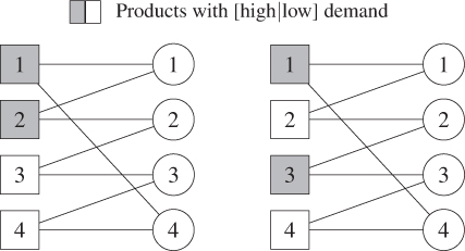
Figure 7.6 Examples of different chaining structures for nonhomogeneous demand case.
PROBLEMS
- 7.1 (Risk‐Pooling Example) Three distribution centers (DCs) each face normally distributed demands, with
 ,
,  , and
, and  . All three DCs have a holding cost of
  and
and  , and all three follow a periodic‐review base‐stock policy using their optimal base‐stock levels.
- Calculate the expected cost of the decentralized system.
- Suppose demands are uncorrelated among the three DCs:
 . Calculate the expected cost of the centralized system.
 - Suppose
 . Calculate the expected cost of the centralized system.
 - Suppose
 ,
,  . Calculate the expected cost of the centralized system.
- 7.2 (No Soup for You) A certain New York City soup vendor sells 15 varieties of soup. The number of customers who come to the soup store on a given day has a Poisson distribution with a mean of 250. A given customer has an equal probability of choosing each of the 15 varieties of soup, and if his or her chosen variety of soup is out of stock (no pun intended), he or she will leave without buying any soup.
You may assume (although it is not necessarily a good assumption) that the demands for different varieties of soup are independent; that is, if the demand for variety i is high on a given day, that doesn't indicate anything about the demand for variety j.
Every type of soup sells for $5 per bowl, and the ingredients for each bowl of soup cost the soup vendor $1. Any soups (or ingredients) that are unsold at the end of the day must be thrown away.
- How many ingredients of each variety of soup should the soup vendor buy? What is the restaurant's total expected underage and overage cost for the day?
- What is the probability that the vendor stocks out of a given variety of soup?
- Now suppose that the soup vendor wishes to streamline his offerings by reducing the selection to 8 varieties of soup. Assume that the total demand distribution does not change, but now the total demand is divided among 8 soup varieties instead of 15. As before, assume that a customer finding his or her choice of soup unavailable will leave without purchasing anything. Now how many ingredients of each variety of soup should the vendor buy? What is the restaurant's total expected underage and overage cost for the day?
- In a short paragraph, explain how this problem relates to risk pooling.
Note: You may use the normal approximation to the Poisson distribution, but make sure to specify the parameters you are using.
- 7.3 (In‐Flight Trash) On a certain airline, the flight attendants collect trash during flights and deposit it all into a single receptacle. Airline management is thinking about instituting an on‐board recycling program in which waste would be divided by the flight attendants and placed into three separate receptacles: one for paper, one for cans and bottles, and one for other trash.
The volume of each of the three types of waste on a given flight is normally distributed. The airline would maintain a sufficient amount of trash‐receptacle space on each flight so that the probability that a given receptacle becomes full under the new system is the same as the probability that the single receptacle becomes full under the old system.
Would the new policy require the same amount of space, more space, or less space for trash storage on each flight? Explain your answer in a short paragraph.
- 7.4 (Days‐of‐Supply Policies) Rather
than setting safety stock levels using base‐stock or
 policies, some companies set their safety stock by requiring a certain number of “days of supply” to be on hand at any given time. For example, if the daily demand has a mean of 100 units, the company might aim to keep an extra 7 days of supply, or 700 units, in inventory. This policy uses
  instead of
  to set safety stock levels.
Consider the N‐DC system described in Section 7.2.1, with independent demands across DCs (
 for
for  ). You may assume that all DCs are identical:
  and
and  for all i. Assume that
  and
and  refer to weekly demands, and that orders are placed by the DCs once per week. Finally, assume that each DC follows a days‐of‐supply policy with k days of supply required to be on hand as safety stock; each DC's order‐up‐to level is then
- Prove that the centralized and decentralized systems have the same amount of total inventory.
- Derive expressions for
 and
and  , the total expected costs of the decentralized and centralized systems. Your expressions may not involve integrals; they may involve the standard normal loss function,
  .
.Hint: Since the DCs are not following the optimal stocking policy, the cost is analogous to (4.29), not to (4.30).
- Prove that
 .
. - Explain in words how to reconcile parts (a) and (c)—how can the centralized cost be smaller even though the two systems have the same amount of inventory?
- 7.5 (Negative Safety Stock) Consider
the N‐DC system described in Section 7.2.1, with independent demands across DCs (
 ). Suppose that the holding cost
is greater than the stockout cost
:
). Suppose that the holding cost
is greater than the stockout cost
:  .
.- Prove that negative safety stock is required at DC i—that the base‐stock level is less than the mean demand.
- Prove that the total inventory (cycle stock and safety stock) required in the decentralized system (each DC operating independently) is less than the total inventory required in the centralized system (all DCs pooled into one). (This is the opposite of the result in Section 7.2.)
- Prove that, despite the result from part (b), the total expected cost of the centralized system is less than that of the decentralized system (
 ).
). - Explain in words how to reconcile parts (b) and (c)—how can it be less expensive to hold more inventory?
- 7.6 (Rationalizing DVR Models) A certain brand of digital video recorder (DVR) is available in three models, one that holds 40 hours of TV programming, one that holds 80 hours, and one that holds 120 hours. The lifecycle for a given DVR model is short, roughly 1 year. Because of long manufacturing lead times, the company must manufacture all of the units it intends to sell before the DVRs go on the market, and it will not have another opportunity to manufacture more before the end of the products' 1‐year life cycles.
Demand for DVRs is highly volatile, and customers are very picky. A customer who wants a given model but finds that it's out of stock will almost never change to a different model—instead, he or she will buy a competitor's product. In this case, the firm incurs both the lost profit and a loss‐of‐goodwill cost. Moreover, any DVRs that are unsold at the end of the year are taken off the market and destroyed, with no salvage value (or cost).
Table 7.2 DVR parameters for Problem 7.6.
Storage Manufacturing Selling Goodwill Mean Annual SD of Annual Space Cost (  )
)Price (  )
)Cost (  )
)Demand (  )
)Demand (  )
)40 80 120 150 40,000 12,000 80 90 150 150 55,000 15,000 120 100 250 150 25,000 8,000 The cost, revenue, and demand parameters for the three models of DVR are given in Table 7.2. Demands are normally distributed with the parameters specified in the table. Moreover, demands for the 80‐ and 120‐hour models are negatively correlated, with a correlation coefficient of
 . (Demands for the 40‐hour model are independent of those for the other two models.)
The company is currently designing its three models for next year, and a very smart supply chain manager noticed that although the models sell for different prices, they cost nearly the same amount to manufacture. The manager thus proposed that the firm manufacture only a single model, containing 120 hours of storage space. When customers purchase a DVR, they specify how much storage space they'd like it to have (either 40, 80, or 120 hours) and pay the corresponding price, and the unit is activated with that much space. If the customer asks for 40 or 80 hours, the remaining storage space simply goes unused. This change can be made with software rather than hardware and therefore costs very little to make.
- Let
 be the quantity of model i manufactured,
  , if the supply chain manager's proposal is not followed. Write the firm's expected profit for model i as a function of
  .
. - Find the optimal order quantities
 and the corresponding total optimal expected profit (for all three models).
 - Let Q be the quantity of the single model manufactured if the manager's proposal is followed. Write the firm's total expected profit as a function of Q. Although it is not entirely accurate to do so, you may assume that the expected selling price for the single model is given by a weighted average of the
 , with weights given by the
  .
. - Find the optimal order quantity Q and the corresponding optimal expected profit. Based on this analysis, should the firm follow the manager's suggestion?
- What other factors should the firm consider before deciding whether to implement the manager's proposal?
- Let
- 7.7 (Proof of Theorem 7.3) Prove Theorem 7.3.
- 7.8 (Transhipment Simulation) Build a spreadsheet simulation model for the two‐retailer transshipment problem from Section 7.4. Your spreadsheet should include columns for the demand at each location; the inventory at each location at the start of the period, before transshipments, and after transshipments; the amount transshipped; and the costs for the period. Assume that demands are Poisson with mean
 per period and that
Use
 and
and  as the base‐stock levels, and assume that both retailers begin the simulation with
  units on‐hand (that is, at the start of period 1, retailer i needs to order
  units to bring its inventory position to
  ).
).- Simulate the system for 500 periods and include the first 10 rows of your spreadsheet in your report.
- Compute the average ordering, transshipment, holding, and penalty costs per period from your simulation.
- Compute the expected transshipment quantity from retailer 1 to retailer 2 (
 ) and the expected ending inventory at retailer 1 (
 ) using 7.8 and 7.9. To compute these quantities, you will need to evaluate some integrals numerically.
 - Compare the results from parts (a) and (c). How closely do the simulated and actual quantities match?
- By trial and error, try to find the values of
 and
and  that minimize the simulated cost. What are the optimal values, and what is the optimal expected cost?
- 7.9 (Binary Transshipments) Consider
the transshipment model from Section 7.4, except now suppose the demands are binary. That is, the demands can only equal 0 or 1, and they are governed by a Bernoulli distribution:
 with probability
  and
and  with probability
  , for
, for  . All of the remaining assumptions from Section 7.4.2 hold.
Your goal in this problem will be to formulate the expected cost and evaluate several feasible values for the base‐stock levels
 . Assume that
  must be an integer.
- Explain why
 .
. - For each possible solution
 below, write the expected values of the state variables
  ,
,  ,
,  , and
, and  , and then write the expected cost
  .
.(The cases in which
 or
or  are similar to the cases above, so we'll skip them.)
Hint 1: If
 , that does not mean that stage i never orders!
Hint 2: To check your cost functions, we'll tell you the following: If
 ,
,  , and
, and  for all
  , then
  ,
,  ,
,  , and
, and  . Note, however, that these parameters do not satisfy the assumptions on page 26.
 -
- Find an instance for which
 . Your instance must satisfy the assumptions on page 26.
 - Find a symmetric instance for which
 . Your instance must satisfy the assumptions on page 26. A symmetric instance is one for which the parameters for the two retailers are identical (
 ,
,  , etc.). (It's a little surprising that a symmetric instance can produce a nonsymmetric solution, but it can.)
 - Prove or disprove the following claim:
 for all instances that satisfy the assumptions on page 26.
- Explain why
- 7.10 (Three‐Stage Flexibility) Consider the three‐stage supply chain flexibility design problem pictured in Figure 7.7.
There are
 products,
  plants, and
  suppliers. In the full‐flexibility structure, each product can be produced at any plant using raw materials sourced from any supplier. We assume that each unit of product consumes one unit of material from each supplier and uses one unit of capacity at each plant. We assume further that the production capacities at the plants are
  ,
,  , and that the suppliers have a limited amount
  of raw materials,
  . The demand for each product is random and is denoted by the random variable
  ,
,  .
.- Derive an expression for the expected sales in the full‐flexibility structure.
- Let
 be a decision variable representing the amount of raw materials from supplier k used to produce product i at plant j. Formulate the flexibility design problem for this three‐stage supply chain.

Figure 7.7 Three‐stage flexibility structure for Problem 7.10.
- 7.11 (Capacity Investment) Recall the formulation of the flexibility design problem 7.32–7.37. Suppose now that the capacity is also a decision, to be made jointly with the network design problem. In particular, the capacities
 are first‐stage decision variables, together with the flexibility investment variables
  . We assume a linear investment cost function for the capacity, with constant marginal investment cost
  per unit.
- Write the new objective function after adding the capacity‐investment cost term.
- Discuss a method for solving this new problem.
- 7.12 (Auto Repair) A small car repair shop has four certified technicians, Irene, Larry, Max, and Suzanne. The shop specializes in four types of vehicles, labeled A, B, C, and D. Each technician has been trained to repair one type of vehicle. On average, the repair of each type of vehicle takes 4 hours. It is estimated that the number of customers who want a type‐A vehicle fixed during a given week is equally likely to be 8, 10, or 12. That is, the probability is
 for each of the possible outcomes, 8, 10, or 12 customers. Each of the other three vehicle types has the same demand distribution for repairs. Furthermore, the demands are iid across time and type. Each technician has a nominal work week of 40 hours at $55 per hour and will be paid for 40 hours even if he or she works fewer than 40 hours in the week. But if a technician works more than 40 hours, then the overtime rate is 150% of the normal pay. The overtime rate applies only to the hours in excess of 40.
- Calculate the expected yearly cost of the dedicated system (in which Irene, Larry, Max, and Suzanne can only service vehicles of type A, B, C, and D, respectively).
- After reading this chapter, the repair shop's manager decides to try a flexible system. Suppose first that the manager uses a chaining structure in which Irene will also be trained to repair type‐B vehicles, Larry to repair type‐C vehicles, Max to repair type‐D vehicles, and Suzanne to repair type‐A vehicles. Calculate the expected yearly cost of overtime for this system.
Note: Given the assumptions made in this problem, for each realization of the random demands, it is possible to calculate the total overtime cost based on the total hours required without determining the assignments of vehicles to technicians.
- Suppose instead that the manager chooses a full‐flexibility system in which every technician is trained to repair all four vehicle models. Calculate the expected yearly cost of overtime for this system.
- Determine the optimal assignment of vehicles to technicians under both the chaining and full flexibility structures if the demands are 12, 8, 10, and 12 for vehicles of types A–D, respectively.
- Suppose the cost of training one technician to repair one new vehicle type is $10,000. What is the expected number of years until the shop recoups the investment cost to convert the dedicated system to the partial flexibility system with the chaining structure? What about the full flexibility system?
- 7.13 (Auto Repair, Part 2) Consider again the auto repair shop in Problem 7.12. Suppose that the number of repairs of type‐A vehicles in a given week has a normal distribution with a mean of 22 and a standard deviation of 3, while the number of repairs of vehicles of types B–D is deterministic and equal to 6 for each type. Calculate the expected yearly cost of overtime for both the chaining structure (as described in Problem 7.12(b)) and the full flexibility system.
Note: Unlike in Problem 7.12, in this problem you must determine the optimal assignment of vehicles to technicians for each realization of the demand in order to calculate the expected overtime cost for the chaining system.
- 7.14 (Max‐Flow Formulation) The production‐allocation problem 7.17–7.21 can also be formulated using a max‐flow formulation.
- Formulate the problem as a max‐flow problem, using the notation already defined in the chapter.
- Research has shown that when demands are independent, chaining can achieve most (roughly 97%) of the benefits of full flexibility as the number of nodes n approaches
 . Show that if the demands are correlated, the situation can be very different.
- 7.15 (Lemma 7.2 Only Holds in Expectation) Develop a counterexample to show that, although Lemma 7.2 holds in expectation, the result does not hold for every individual demand instance.