Chapter 6
Multiechelon InventoryModels
6.1 Introduction
In this chapter, we study inventory optimization models for multiechelon (or multistage) systems with shipments made among the stages. There are two common ways to interpret the stages or nodes in a multiechelon system:
- Stages represent locations in a supply chain network, and links among the stages represent physical shipments of goods. For example, the stages in Figure 6.1(a) may represent the following physical locations: a supplier in China, a factory in California, a warehouse in Chicago, and a retailer in Detroit (respectively).
- Stages represent processes that the product must undergo during manufacturing, assembly, and/or distribution. Links among the stages represent transitions between steps in the process. For example, the stages in Figure 6.1(a) may represent the following processes: manufacturing, assembly, testing, and packaging. These four functions may take place in four different locations or all within the same building—it is largely irrelevant from the perspective of the model. We sometimes refer to the stages as different “products,” even if they really represent different phases of producing a single product.
Either interpretation is acceptable for the models that we discuss, although some models are more naturally interpreted in one way than the other. In the discussion that follows, we will use terms such as “shipped” or “transferred” under either interpretation to mean “moved from one stage to the next.”
6.1.1 Multiechelon Network Topologies
Multiechelon networks can be structured in a number of ways, and the network's topology plays a large role in determining how the system is analyzed and optimized. The simplest multiechelon topology is a serial system (or series system), in which each echelon contains exactly one stage. Put another way, every stage has exactly one predecessor and exactly one successor, except for two stages, one of which has exactly one successor and no predecessors, and the other of which has exactly one predecessor and no successors. (A predecessor of stage j is another stage that ships product to j, and a successor of j is another stage that j ships to.) See Figure 6.1(a) for an example of a serial system.

Figure 6.1 Multiechelon network topologies.
In an assembly system, each stage has at most one successor; see Figure 6.1(b). Interpretation (2) is most common for assembly systems: The network represents a bill‐of‐materials structure that describes how a final product is assembled from raw materials and intermediate products. In this case, the links in the network indicate “and” relationships: To make one unit of the product at stage j, we need one (or more) unit of each of j's predecessors. Assembly systems can also be viewed under interpretation (1), with links denoting the geographic flow of materials. If stage j has three predecessors, then there are three stages that make the product and ship it to stage j. Here, too, links represent “and” relationships since all three upstream stages ship product to stage j. An alternate, but less common, way to use interpretation (1) is that the links represent “or” relationships, and stage j's predecessors are multiple alternate suppliers from which stage j can order. In a given order cycle, it may order from one, more than one, or all of its predecessors, depending on their capacities, the observed demands, and so on. Under any of these interpretations, assembly systems are commonly used to model upstream portions of supply chains whose purpose is to consolidate products or locations into a few stages.
A distribution system (Figure 6.1(c)) is the opposite of an assembly system: Each stage has at most one predecessor. Interpretation (1) is most common for distribution systems, which are often used to model downstream portions of supply chains—the portion that moves material from a few centralized locations to a set of retailers or customers distributed throughout a large geographical region.
Tree systems (Figure 6.1(d)) are hybrids of assembly and distribution systems—each stage may have multiple predecessors and successors—but tree systems may contain no undirected cycles. (A cycle, in graph theory, is a portion of the graph whose links allow one to move from a starting node, through a sequence of other nodes, and back to the starting node, without repeating any other nodes links. An undirected cycle is a cycle in the graph that results from removing all of the arrows from the links so that movement can go in either direction.) Finally, general systems allow any number of successors and predecessors and have no restrictions on undirected cycles. Figure 6.1(e) shows an example. General systems are the most flexible topology but are also the most difficult to analyze andoptimize.
6.1.2 Stochastic vs. Guaranteed Service
The most challenging aspect of multiechelon inventory models is that a given stage j provides stochastic lead times to its successors, even if the transportation lead time is deterministic, due to occasional stockouts at stage j, and the optimal inventory parameters at stage j's successors depend on the probability distributions of these stochastic lead times. We have discussed some results for optimizing single‐stage systems with stochastic lead times (see, e.g., Section 5.3.3), but in those models, we assume the lead‐time distributions are known and that the lead times are iid. In contrast, the probability distributions of the lead times in multiechelon systems are very complex and difficult to characterize, the lead times are not iid, and moreover, the distributions depend on the upstream inventory parameters. Even for single‐stage systems, the distributions of the lead times generated by the stage are quite complex (Higa et al., 1975; Sherbrooke, 1975).
Twoprimary types of models have been developed to handle these complexities in multiechelon base‐stock systems: stochastic‐service models and guaranteed‐service models (Graves and Willems, 2003a). In stochastic‐service models, each stage i sets a base‐stock level![]() and meets demand from stock whenever possible using this base‐stock level. The actual lead time seen by downstream stages is stochastic since some demands will be backordered. This is the approach taken in the seminal model of Clark and Scarf (1960) and related works, discussed in Section 6.2.
and meets demand from stock whenever possible using this base‐stock level. The actual lead time seen by downstream stages is stochastic since some demands will be backordered. This is the approach taken in the seminal model of Clark and Scarf (1960) and related works, discussed in Section 6.2.
In guaranteed‐service models, stage i sets a “committed service time” (CST), denoted ![]() , within which it is required to satisfy every demand.
1
For example, if
, within which it is required to satisfy every demand.
1
For example, if ![]() 5 periods, then every demand must be satisfied in no more than 5 periods. To make this guarantee, guaranteed‐service models require the demand to be bounded above. The guaranteed‐service assumption provides the strategic safety stock placement problem (SSSPP), described in Section 6.3, its tractability. There is a close relationship between the CST and the base‐stock level, since a larger base‐stock level allows the stage to quote a shorter CST. In fact, any given set of CSTs implies a certain set of base‐stock levels, and the base‐stock levels, not the CSTs, are usually the main quantities of interest.
5 periods, then every demand must be satisfied in no more than 5 periods. To make this guarantee, guaranteed‐service models require the demand to be bounded above. The guaranteed‐service assumption provides the strategic safety stock placement problem (SSSPP), described in Section 6.3, its tractability. There is a close relationship between the CST and the base‐stock level, since a larger base‐stock level allows the stage to quote a shorter CST. In fact, any given set of CSTs implies a certain set of base‐stock levels, and the base‐stock levels, not the CSTs, are usually the main quantities of interest.
One way to view the difference between these two approaches is that guaranteed‐service models allow a CST of ![]() but require a service level of
but require a service level of ![]() while stochastic‐service models assume a service time of
while stochastic‐service models assume a service time of ![]() but allow a less restrictive service level of
but allow a less restrictive service level of ![]() . Another interpretation is that stockouts in stochastic‐service models incur a penalty that is proportional to the time the unit is backordered, whereas in guaranteed‐service models, no penalty is incurred until the backorder has lasted
. Another interpretation is that stockouts in stochastic‐service models incur a penalty that is proportional to the time the unit is backordered, whereas in guaranteed‐service models, no penalty is incurred until the backorder has lasted ![]() periods, and after that the penalty is
periods, and after that the penalty is ![]() . (See Figure 6.2.) In fact, in guaranteed‐service models, a backorder isn't really even considered a backorder until it has lasted
. (See Figure 6.2.) In fact, in guaranteed‐service models, a backorder isn't really even considered a backorder until it has lasted ![]() periods.
periods.

Figure 6.2 Interpretation of stockout penalties.
It is important to remember that these are both merely mathematical models, two different ways to describe the mechanics and the optimization problem underlying a multiechelon inventory system. The end result of either approach is a set of base‐stock levels, even though the decision variables in the guaranteed‐service model are the CSTs rather than base‐stock levels. Thus, the guaranteed‐service model can be used even when stages do not actually quote CSTs to one another. Either modeling approach can be used to model a given system, and the choice of approach is a modeling decision with pros and cons just like any other.
In Section 6.2, we first discuss stochastic‐service models, describing an optimal and a heuristic approach for optimizing base‐stock levels in serial systems and then briefly discussing the extent to which these methods can be extended to solve assembly and distribution systems. Then, in Section 6.3, we discuss guaranteed‐service models, beginning with an analysis of single‐stage systems and working our way up to tree systems.
See van Houtum et al. (1996) and Graves and Willems (2003a) (among others) for further reviews of the literature on stochastic‐ and guaranteed‐service models,respectively.
6.2 Stochastic‐ServiceModels
6.2.1 Serial Systems
Consider an N‐stage serial system, with the stages labeled as in Figure 6.3. Stage 1 is farthest downstream. It faces stochastic external customer demand and places replenishment orders to stage 2, which places replenishment orders to stage 3, and so on up the line to stage N. Stage N, in turn, places replenishment orders to an external supplier that is assumed to have infinite supply.
We consider a continuous‐review, infinite‐horizon system, though nearly all of the results described below hold (with slight modifications) for periodic‐review systems, as well. Orders placed by stage j incur a transportation lead time of ![]() ; that is, the order is received
; that is, the order is received ![]() time units later if stage
time units later if stage ![]() had sufficient stock to ship the order immediately, and more than
had sufficient stock to ship the order immediately, and more than ![]() time units later otherwise. Stage j incurs a holding cost of
time units later otherwise. Stage j incurs a holding cost of ![]() per item per time unit, which is charged on the on‐hand inventory at stage j as well as on the inventory in transit to stage
per item per time unit, which is charged on the on‐hand inventory at stage j as well as on the inventory in transit to stage ![]() . (One can show that the expected number of units in transit is a constant, and therefore the in‐transit holding cost does not affect the optimization.) Unmet demands are backordered at all stages, but only stage 1 incurs a stockout cost, given by p per item per time unit. There are no fixed costs, and we will ignore any per‐unit ordering costs.
. (One can show that the expected number of units in transit is a constant, and therefore the in‐transit holding cost does not affect the optimization.) Unmet demands are backordered at all stages, but only stage 1 incurs a stockout cost, given by p per item per time unit. There are no fixed costs, and we will ignore any per‐unit ordering costs.

Figure 6.3 N‐stage serial system in stochastic‐service model.
In multiechelon inventory theory, the echelon of stage j (or just “echelon j”) is defined as the set of stages ![]() ; that is, the set that includes j and all downstream stages. Note that this is a particular inventory‐theoretic use of the term “echelon” and is different from the way we defined it in Chapter 1. Stage j's echelon inventory is the total inventory in echelon j, and its local inventory is the inventory at stage j only. It turns out to be more convenient to optimize stage j's echelon inventory rather than its local inventory.
; that is, the set that includes j and all downstream stages. Note that this is a particular inventory‐theoretic use of the term “echelon” and is different from the way we defined it in Chapter 1. Stage j's echelon inventory is the total inventory in echelon j, and its local inventory is the inventory at stage j only. It turns out to be more convenient to optimize stage j's echelon inventory rather than its local inventory.
Stage j's local on‐hand inventory, denoted ![]() , includes items on hand at stage j only, whereas stage j's echelon on‐hand inventory, denoted
, includes items on hand at stage j only, whereas stage j's echelon on‐hand inventory, denoted ![]() , includes all of the on‐hand inventory in echelon j, plus all of the in‐transit inventory among these stages:
, includes all of the on‐hand inventory in echelon j, plus all of the in‐transit inventory among these stages:

where ![]() is the inventory in transit from i to
is the inventory in transit from i to ![]() , and
, and ![]() . Stage j's local and echelon inventory levels, denoted
. Stage j's local and echelon inventory levels, denoted ![]() and
and ![]() , respectively, are given by
, respectively, are given by
where ![]() is the (local) backorders at stage 1. Note that the local inventory level at stage j subtracts the backorders at stage j while the echelon inventory level subtracts those at stage 1; upstream backorders are not counted in
is the (local) backorders at stage 1. Note that the local inventory level at stage j subtracts the backorders at stage j while the echelon inventory level subtracts those at stage 1; upstream backorders are not counted in ![]() , and therefore the echelon inventory level does not equal the sum of the local quantities.
, and therefore the echelon inventory level does not equal the sum of the local quantities.
The holding cost ![]() is called a local holding cost, and it is charged based on the number of items in stage j's local inventory plus the number of items in transit from stage j to
is called a local holding cost, and it is charged based on the number of items in stage j's local inventory plus the number of items in transit from stage j to ![]() ,
, ![]() . We will mostly work with stage j's echelon holding cost, denoted
. We will mostly work with stage j's echelon holding cost, denoted ![]() and defined as
and defined as
(with ![]() ). Typically, local holding costs increase as we move downstream in the supply chain since value is added to the product at each stage. Therefore,
). Typically, local holding costs increase as we move downstream in the supply chain since value is added to the product at each stage. Therefore, ![]() represents the holding cost corresponding to the value added at stage j. It turns out that we can calculate total holding costs using either echelon or local quantities:
represents the holding cost corresponding to the value added at stage j. It turns out that we can calculate total holding costs using either echelon or local quantities:
The following theorem establishes the form of the optimal inventory policy for serial systems. It was proved for finite‐horizon problems in the seminal paper of Clark and Scarf (1960) and for infinite‐horizon problems by Federgruen and Zipkin (1984).
In an echelon base‐stock policy, each stage j has a fixed level ![]() , called the echelon base‐stock level, and it places an order as needed to bring its echelon inventory position (defined as stage j's echelon inventory level,
, called the echelon base‐stock level, and it places an order as needed to bring its echelon inventory position (defined as stage j's echelon inventory level,![]() , plus any items on‐order from stage
, plus any items on‐order from stage ![]() ) equal to
) equal to ![]() . An echelon base‐stock policy is essentially the same as the base‐stock policies we are already familiar with except that it is the echelon inventory, rather than the local inventory, that we compare to the base‐stock level when making ordering decisions. We use
. An echelon base‐stock policy is essentially the same as the base‐stock policies we are already familiar with except that it is the echelon inventory, rather than the local inventory, that we compare to the base‐stock level when making ordering decisions. We use ![]() to denote the vector of echelon base‐stock levels, one for each stage.
to denote the vector of echelon base‐stock levels, one for each stage.
We will discuss approaches for finding optimal or near‐optimal echelon base‐stock levels. Local base‐stock levels (denoted ![]() ) can be obtained from the echelon base‐stock levels by setting
) can be obtained from the echelon base‐stock levels by setting
defining ![]() . (This assumes that
. (This assumes that ![]() . If not, we let
. If not, we let ![]() and set
and set ![]() , again setting
, again setting ![]() .) And echelon base‐stock levels can be obtained from local onesas follows:
.) And echelon base‐stock levels can be obtained from local onesas follows:

Let ![]() be a random variable representing the lead‐time demand at stage j. Since stage j's demands are ultimately generated by the external customer (via orders placed to stage 1, then to stage 2, and so on), stage j's demand per time unit has the same distribution as the customer's demand, but the distribution of stage j's lead‐time demand
be a random variable representing the lead‐time demand at stage j. Since stage j's demands are ultimately generated by the external customer (via orders placed to stage 1, then to stage 2, and so on), stage j's demand per time unit has the same distribution as the customer's demand, but the distribution of stage j's lead‐time demand ![]() depends on
depends on ![]() . Let
. Let ![]() be the cdf of
be the cdf of ![]() .
.
Table 6.1 summarizes the notation for the stochastic‐service model.
Table 6.1 Stochastic‐service model notation summary.
Formula for ![]() assumes
assumes ![]() ; see page 19.
; see page 19.
6.2.2 Exact Approach for Serial Systems
For a given set of base‐stock levels, the expected cost of the system can be expressed using either local or echelon quantities:


(Note that the prime in ![]() indicates local quantities, not a derivative.) These two expressions are equivalent (see Problem 6.5), but 6.9 will be more convenient for us to work with.
indicates local quantities, not a derivative.) These two expressions are equivalent (see Problem 6.5), but 6.9 will be more convenient for us to work with.
We wish to choose ![]() to minimize
to minimize ![]() .
. ![]() is a messy function of
is a messy function of ![]() because the inventory levels on the right‐hand side depend on
because the inventory levels on the right‐hand side depend on ![]() in messy ways. In fact, since
in messy ways. In fact, since ![]() affects the inventory levels at all stages downstream from j, it would seem that we need to jointly optimize all of the
affects the inventory levels at all stages downstream from j, it would seem that we need to jointly optimize all of the ![]() simultaneously. Fortunately, a much simpler and more elegant procedure suffices.
simultaneously. Fortunately, a much simpler and more elegant procedure suffices.
Let ![]() be the echelon inventory–transit position at stage j, which equals the echelon inventory level at j plus all items in transit from stage
be the echelon inventory–transit position at stage j, which equals the echelon inventory level at j plus all items in transit from stage ![]() :
:
That is, ![]() includes all items that have been ordered from
includes all items that have been ordered from ![]() but not yet received, whereas
but not yet received, whereas ![]() only includes items that have been shipped. The difference between the two equals the number of backorders at
only includes items that have been shipped. The difference between the two equals the number of backorders at ![]() (i.e.,
(i.e., ![]() ), and they are equal if there are no backorders at
), and they are equal if there are no backorders at ![]() .
.
The conservation‐of‐flow argument from Section 4.3.4.1 can be applied here to show that
since all items that were shipped from ![]() at or before period t have arrived by period
at or before period t have arrived by period ![]() , no items that were shipped after t have arrived, and the intervening demand is
, no items that were shipped after t have arrived, and the intervening demand is ![]() . This equation is similar to (4.41), except that the inventory position is replaced by the inventory–transit position.
2
In the single‐stage models in Chapters 4 and 5, the supplier never has stockouts, so
. This equation is similar to (4.41), except that the inventory position is replaced by the inventory–transit position.
2
In the single‐stage models in Chapters 4 and 5, the supplier never has stockouts, so ![]() and
and ![]() are equal.
are equal.
One can show that
Intuitively, 6.13 says that the inventory at or en route to echelon j equals the echelon base‐stock level at j, unless the upstream inventory is insufficient to attain the base‐stock level, in which case it equals the upstream inventory level. For a more rigorous proof, see Problem 6.14.
In addition, note that at stage N,
for all t, since the upstream supplier to stage N never has stockouts.
In steady state, we can rewrite 6.12, 6.13, and 6.14 as
Equations 6.15–6.17 provide a recursion that expresses ![]() in terms of
in terms of ![]() ,
, ![]() in terms of
in terms of ![]() , and so on, until we reach
, and so on, until we reach ![]() , which equals a constant.
, which equals a constant.
We next introduce three auxiliary functions that condition the expected cost of the system on the state variables in the recursion. These functions will allow us to develop a recursion for the (unconditional) expected cost for a given vector ![]() of base‐stock levels, and then to find the optimal base‐stock vector.
of base‐stock levels, and then to find the optimal base‐stock vector.


Each auxiliary function fixes one of the recursion variables—![]() ,
, ![]() , or
, or ![]() —and then calculates the expected cost in stages
—and then calculates the expected cost in stages ![]() using that value as the starting point. For example, suppose we have a 4‐stage system with base‐stock vector
using that value as the starting point. For example, suppose we have a 4‐stage system with base‐stock vector ![]() and we know that
and we know that ![]() . Then the expected cost for stages 1 and 2 is given by
. Then the expected cost for stages 1 and 2 is given by ![]() . Similarly, the expected cost in stages 1 and 2 is
. Similarly, the expected cost in stages 1 and 2 is ![]() if we know that
if we know that ![]() and is
and is ![]() if we know that
if we know that ![]() .
.
We can write 6.18–6.20 recursively. First let
Then

Similarly,

where the expectation is over ![]() . (The second equality follows from 6.16.) And,
. (The second equality follows from 6.16.) And,

where the second equality follows from 6.17. Continuing this process, we get

and so on.
In general, for ![]() , given
, given ![]() , we have:
, we have:
So for any base‐stock vector ![]() and any known value of
and any known value of ![]() ,
, ![]() , or
, or ![]() , we can calculate the expected cost in stages
, we can calculate the expected cost in stages ![]() . What's more, we know
. What's more, we know ![]() for
for ![]() —it equals
—it equals ![]() . Therefore, the expected cost of the entire system,
. Therefore, the expected cost of the entire system, ![]() , is given by
, is given by ![]() .
.
This gives us a way to calculate the expected cost recursively for a given
![]() . We are only a short leap from finding the optimal
. We are only a short leap from finding the optimal
![]() . Since the recursion for stages
. Since the recursion for stages ![]() does not depend on
does not depend on ![]() , we don't need to choose
, we don't need to choose ![]() until we reach
until we reach ![]() in the recursion. At that point, we can simply set
in the recursion. At that point, we can simply set ![]() to the y that minimizes
to the y that minimizes ![]() . This idea is made concrete in the next theorem. Note that the functions in the theorem omit “
. This idea is made concrete in the next theorem. Note that the functions in the theorem omit “![]() ” since we are choosing
” since we are choosing ![]() rather than evaluating the cost for a given
rather than evaluating the cost for a given ![]() .
.
Theorem 6.2 is the result of the groundwork laid by Clark and Scarf (1960) and subsequent refinements by Chen and Zheng (1994). It says that, rather than simultaneously optimizing all of the base‐stock levels, we can optimize them sequentially, beginning with stage 1 and working upstream, one stage at a time. Moreover, ![]() is known to be convex, so at each iteration we only need to minimize a single‐variable, convex function. This theorem underlies much of the theory of multiechelon stochastic‐service models. (Zipkin (2000) even goes so far as to call 6.24–6.27 the “fundamental equation[s] of supply‐chain theory.”)
is known to be convex, so at each iteration we only need to minimize a single‐variable, convex function. This theorem underlies much of the theory of multiechelon stochastic‐service models. (Zipkin (2000) even goes so far as to call 6.24–6.27 the “fundamental equation[s] of supply‐chain theory.”)
The arguments above imply that, to evaluate the cost of a given (not necessarily optimal) base‐stock vector ![]() , we simply skip the optimization step 6.26 and evaluate the functions using
, we simply skip the optimization step 6.26 and evaluate the functions using ![]() instead of
instead of ![]() .
.
Consider the optimization problem at stage 1. We have:

This function is identical in form to the newsvendor objective function (4.3), with p replaced by ![]() . Therefore, from (4.17),
. Therefore, from (4.17), ![]() is minimized by
is minimized by

At upstream stages, the functions ![]() become more complicated and cannot be minimized in closed form. In fact, the expectation in
become more complicated and cannot be minimized in closed form. In fact, the expectation in ![]() must be evaluated numerically for every candidate value y. Therefore, although 6.26 is a convex minimization problem, it is somewhat computationally expensive to execute, as well as cumbersome to implement.
must be evaluated numerically for every candidate value y. Therefore, although 6.26 is a convex minimization problem, it is somewhat computationally expensive to execute, as well as cumbersome to implement.
The function ![]() is similar to a deterministic cost function, analogous to (4.1) or (5.3)—if we know that
is similar to a deterministic cost function, analogous to (4.1) or (5.3)—if we know that ![]() at a given time, then the cost rate at that time for stages
at a given time, then the cost rate at that time for stages ![]() is
is ![]() . For
. For ![]() , 6.28 shows that the form of
, 6.28 shows that the form of ![]() is exactly the same as that of (4.1) or (5.3) since
is exactly the same as that of (4.1) or (5.3) since
For ![]() ,
, ![]() replaces the stockout penalty term. In fact,
replaces the stockout penalty term. In fact, ![]() is sometimes called the implicit penalty function. It captures the downstream implications of upstream stockouts.
is sometimes called the implicit penalty function. It captures the downstream implications of upstream stockouts.
6.2.3 Heuristic Approach for SerialSystems
Suppose we have found ![]() , and we now need to find
, and we now need to find ![]() . Theorem 6.2 tells us that
. Theorem 6.2 tells us that ![]() does not depend on the base‐stock levels at stages
does not depend on the base‐stock levels at stages ![]() , although it does indirectly depend on the echelon holding costs at those stages (because
, although it does indirectly depend on the echelon holding costs at those stages (because ![]() includes
includes ![]() ). Suppose we truncate the system at stage j (i.e., remove all stages upstream from j), leave the echelon holding costs at the remaining stages intact, and replace p with
). Suppose we truncate the system at stage j (i.e., remove all stages upstream from j), leave the echelon holding costs at the remaining stages intact, and replace p with ![]() . Then the
. Then the ![]() that is optimal for stage j in this truncated system is also optimal for stage j in the original system (Shang and Song, 2003). In other words, the y that minimizes
that is optimal for stage j in this truncated system is also optimal for stage j in the original system (Shang and Song, 2003). In other words, the y that minimizes

also minimizes ![]() in 6.26. (In 6.31 we have emphasized that
in 6.26. (In 6.31 we have emphasized that ![]() and
and ![]() are functions of y, and we have truncated the system at j; otherwise, it is identical to 6.8.) We obtained a similar result for stage 1 in 6.29.
are functions of y, and we have truncated the system at j; otherwise, it is identical to 6.8.) We obtained a similar result for stage 1 in 6.29.
Why is this true? Well, in the truncated system, each unit sold reduces the holding cost by ![]() , but the true cost reduction, for the original system, is
, but the true cost reduction, for the original system, is ![]() . Therefore, there is an extra
. Therefore, there is an extra ![]() in “perceived benefit” for each sale that is not reflected in the holding costs of the truncated system. Similarly, each demand that cannot be satisfied immediately increases the cost by this amount. We therefore model this by adding the perceived benefit,
in “perceived benefit” for each sale that is not reflected in the holding costs of the truncated system. Similarly, each demand that cannot be satisfied immediately increases the cost by this amount. We therefore model this by adding the perceived benefit, ![]() , to the original stockout cost, p.
, to the original stockout cost, p.
Now, 6.31 is no easier to solve than 6.26—except for one special case. Suppose that ![]() , for some fixed
, for some fixed ![]() . (Or, equivalently,
. (Or, equivalently, ![]() and
and ![]() .) Then it is optimal to hold all of the inventory at stage 1, because upstream inventory is not cheaper, and it requires a longer lead time to reach the customer. We can therefore replace this j‐stage system with a single‐stage system with a holding cost of
.) Then it is optimal to hold all of the inventory at stage 1, because upstream inventory is not cheaper, and it requires a longer lead time to reach the customer. We can therefore replace this j‐stage system with a single‐stage system with a holding cost of ![]() , a stockout cost of
, a stockout cost of ![]() , and a lead time of
, and a lead time of ![]() .
.
This would make the problem easy to solve, but would the solution help us? It turns out that, if we choose good values for ![]() , the resulting cost functions provide bounds on the actual cost function, and the resulting base‐stock levels provide bounds on the optimal base‐stock levels. Moreover, these bounds can be used to compute heuristic values for
, the resulting cost functions provide bounds on the actual cost function, and the resulting base‐stock levels provide bounds on the optimal base‐stock levels. Moreover, these bounds can be used to compute heuristic values for ![]() , which turn out to be remarkably accurate. This approximation was proposed by Shang and Song (2003).
, which turn out to be remarkably accurate. This approximation was proposed by Shang and Song (2003).
We consider two different values for ![]() . Let
. Let ![]() be the cost function 6.31 with
be the cost function 6.31 with ![]() replaced by
replaced by ![]() for all i, and let
for all i, and let ![]() be the same function with
be the same function with ![]() replaced by
replaced by ![]() for all i. Let
for all i. Let ![]() be the lead‐time demand for a single‐stage system with lead time
be the lead‐time demand for a single‐stage system with lead time ![]() , i.e.,
, i.e.,

and let ![]() be its cdf.
be its cdf.
Then the functions ![]() and
and ![]() are minimized by
are minimized by

and

respectively.
The theorem suggests that we can approximate ![]() , for each j, using a weighted average of
, for each j, using a weighted average of ![]() and
and ![]() . In fact, Shang and Song (2003) suggest using a simple average, that is,
. In fact, Shang and Song (2003) suggest using a simple average, that is,

If local base‐stock levels are desired, we can compute ![]() from S˜j as described in Section 6.2.1.
from S˜j as described in Section 6.2.1.
This approximation performs quite well: Shang and Song (2003) report an average error of 0.24% and a maximum error of less than 1.5% on their test instances, where the errors are computed by comparing the heuristic solutions with the exact solutions from Theorem 6.2.
This heuristic can be used for periodic‐review systems as well. However, in this case, the lead‐times must each be inflated by one unit, assuming the system uses the sequence of events on page 90. See Shang and Song (2003)for details.
6.2.4 Other Network Topologies
Assembly Systems: Assembly systems turn out to be easy to solve—or, at least, no harder than serial systems. Rosling (1989) proves that every assembly system can be transformed to an equivalent serial system. That serial system can be solved using any method available for such systems (for example, the exact method in Section 6.2.2 or the heuristic one in Section 6.2.3). The resulting solution can then be transformed back to a solution for the assembly system. The equivalence between the two systems is exact, meaning that if we solve the serial system optimally, then the transformed solution will be optimal for the assembly system.
Distribution Systems: Unfortunately, distribution systems are much more difficult. In part, the difficulty stems from the fact that, if a given stage has insufficient inventory to meet the orders placed by its successors, it must decide how to allocate the inventory that it does have among them. For example, it may assign items first‐come, first‐served, or randomly, or based on some priority system. Therefore, in addition to choosing a replenishment policy at each node, we must also choose an allocation policy. Under stochastic demands, even the optimal form of these policies is unknown, let alone the optimal parameters for the policies. Usually, we simply choose a plausible ordering policy (e.g., a base‐stock policy) and a plausible allocation policy (e.g., a first‐come, first‐served policy) and then optimize the parameters under those assumptions.
The simplest type of distribution system is the one‐warehouse, multiple‐retailer (OWMR) system, a two‐echelon system with one upstream stage (the “warehouse”) and several downstream stages (the “retailers”). The best known exact algorithm for OWMR systems is the projection algorithm (Graves, 1985; Axsäter, 1990), which involves iterating over the possible values for ![]() (the warehouse base‐stock level). For each possible value of
(the warehouse base‐stock level). For each possible value of ![]() , we can find the corresponding optimal
, we can find the corresponding optimal ![]() for the retailers by solving a single‐variable, convex optimization problem for each j. However, the total cost is not a convex function of
for the retailers by solving a single‐variable, convex optimization problem for each j. However, the total cost is not a convex function of ![]() , which means that we must perform an exhaustive search to find
, which means that we must perform an exhaustive search to find ![]() . Moreover, each evaluation of the objective function requires numerical convolution, a computationally costly calculation.
. Moreover, each evaluation of the objective function requires numerical convolution, a computationally costly calculation.
Several heuristics have been proposed for OWMR and more general distribution systems. Sherbrooke (1968) proposed the so‐called “METRIC” model; his method approximates the stochastic lead times generated by the warehouse for the retailers by replacing them with their means. Graves (1985) proposes a two‐moment approximation in which a messy distribution necessary to evaluate the cost is replaced by a simpler distribution with the same mean and variance. This approach can also be used to approximate serial systems. Gallego et al. (2007) propose the “restriction–decomposition” heuristic, which involves solving three subheuristics, each of which makes some simplifying assumption to render the model tractable, and then taking the best of the three resulting solutions. Özer and Xiong (2008) propose a heuristic in which the distribution system is decomposed into multiple serial systems, each of which is solved independently, and then the solutions from the serial systems are summed to obtain a solution for the distribution system. A similar approach is used in the “decomposition–aggregation” heuristic by Rong et al. (2017a), which uses a procedure they call “backorder matching” to convert the base‐stock levels from the serial system into those for the distribution system. They also propose a more accurate, but more computationally intensive, procedure, called the “recursive optimization” heuristic, which is inspired byTheorem 6.2.
Tree and General Systems: Given the difficulty of solving distribution systems, these more general systems have received little attention in the literature. See, for example, de Kok and Visschers (1999)and de Kok and Fransoo (2003).
6.3 Guaranteed‐ServiceModels
6.3.1 Introduction
Figure 6.6 depicts the supply chain for a digital camera made by Kodak. Each stage represents an activity (as in interpretation (2) from Section 6.1): either a processing activity such as packaging or testing, or an assembly activity such as combining a wafer and an “imager base” to construct an “imager assembly.” These activities may occur at different locations or together at the same location. Each stage functions as an autonomous unit that can hold safety stock, place orders to upstream stages, and so on.

Figure 6.6 Digital camera supply chain network..
Reprinted by permission, Graves and Willems, Optimizing strategic safety stock placement in supply chains, Manufacturing and Service Operations Management, 2(1), 2000, 68–83. ©2000, the Institute for Operations Research and the Management Sciences (INFORMS), 7240 Parkway Drive, Suite 300, Hanover, MD 21076 USA
The question of interest here is, which stages should hold safety stock, and how much? It may not be necessary for all stages to hold safety stock, but only a few. These stages serve as buffers to absorb all of the demand uncertainty in the supply chain. This problem is a strategic one, since the location of safety stock is a design problem that is costly to change frequently. This problem is therefore known as the strategic safety stock placement problem (SSSPP).
The supply chain operates in an infinite‐horizon, periodic‐review setting, and each stage follows a base‐stock policy. Each stage quotes a lead time, or committed service time (CST), to its downstream stage(s) within which it promises to deliver each order. As we will see, there is a direct relationship between the CST and the safety stock (and base‐stock level) required at each stage. The goal of the strategic safety stock placement model is to choose the CST (and, therefore, the safety stock and base‐stock level) at each stage in order to minimize the expected holding cost in each period.
Each stage is required to provide 100% service to its downstream stage(s). In other words, each stage is obligated to deliver every order within the CST regardless of the size of the order. In order to enforce this restriction, we will have to assume that the demand is bounded. We will discuss this assumption further in Section 6.3.2.
The guaranteed‐service assumption was first used by Kimball in 1955 (later reprinted as Kimball, 1988). Simpson (1958) applied it to serial systems and Graves (1988) discussed how to solve the resulting safety stock optimization problem. Inderfurth (1991), Minner (1997), and Inderfurth and Minner (1998) discuss dynamic programming (DP) approaches for distribution and assembly systems. Graves and Willems (2000) extend this to tree systems, and Magnanti et al. (2006) and Humair and Willems (2011) allow general networks that include (undirected) cycles.
We will build gradually to tree networks similar to the one pictured in Figure 6.6, considering first the single‐stage case, then serial systems, and finally tree networks. First, we will discuss the demand process.
Throughout Section 6.3, ![]() will be used to represent the local holding cost at stage i. (In Section 6.2, it represented the echelon holding cost.)
will be used to represent the local holding cost at stage i. (In Section 6.2, it represented the echelon holding cost.)
6.3.2 Demand
Weassume that the demand in any interval of time is bounded. In practice, this is not a terribly realistic assumption (unless the bound is very large), but it is necessary in this model to guarantee 100% service. One way to model the demand is simply to truncate the right tail of the demand distribution. That is, if demand is normally distributed, we simply ignore any demands greater than, say, ![]() standard deviations above the mean, for some constant
standard deviations above the mean, for some constant ![]() . This is the approach we will take throughout.
. This is the approach we will take throughout.
In particular, consider a stage that faces external demand (as opposed to serving other downstream stages). Suppose the demand per period is distributed ![]() . Then we will assume that the total demand in any
. Then we will assume that the total demand in any ![]() periods is bounded by
periods is bounded by
for some constant ![]() . In other words, we assume that the demand in
. In other words, we assume that the demand in ![]() consecutive periods is no more than
consecutive periods is no more than ![]() standard deviations above its mean, since the mean demand in
standard deviations above its mean, since the mean demand in ![]() periods is
periods is ![]() and the standard deviation is
and the standard deviation is ![]() . This implies that the demand in a single period is bounded by
. This implies that the demand in a single period is bounded by ![]() . The reverse implication, however, is not true: Assuming the single‐period demand is bounded by
. The reverse implication, however, is not true: Assuming the single‐period demand is bounded by ![]() implies that the
implies that the ![]() ‐period demand is bounded by
‐period demand is bounded by ![]() ; it does not imply the stronger bound of
; it does not imply the stronger bound of ![]() .
.
If, in actuality, the demand in a given ![]() ‐period interval exceeds
‐period interval exceeds ![]() , the excess demands are assumed to be handled in some other manner—say, by outsourcing, scheduling overtime shifts, or by some other method not captured in the model. This allows us to ignore the demands in the tail and pretend the demand never exceeds its bound.
, the excess demands are assumed to be handled in some other manner—say, by outsourcing, scheduling overtime shifts, or by some other method not captured in the model. This allows us to ignore the demands in the tail and pretend the demand never exceeds its bound.
We will use the demand bound in 6.33, but any other bound ![]() is acceptable, with suitable changes to the derivations below.
is acceptable, with suitable changes to the derivations below.
6.3.3 Single‐StageNetwork
Consider a single stage that quotes a CST of ![]() periods to an external customer. (Recall that S denotes a CST in this section, but a base‐stock level in Section 6.2.) The stage receives raw materials from an external supplier, which promises an inbound CST of
periods to an external customer. (Recall that S denotes a CST in this section, but a base‐stock level in Section 6.2.) The stage receives raw materials from an external supplier, which promises an inbound CST of ![]() periods. Finally, the stage itself requires a processing time of T periods to perform its function. Items that have been ordered from the supplier but not yet received are referred to as on‐order inventory; those that have been received from the supplier and are currently being processed are referred to as work‐in‐progress (WIP) inventory; and those that have completed their processing are referred to as finished‐goods inventory. (See Figure 6.7.)
periods. Finally, the stage itself requires a processing time of T periods to perform its function. Items that have been ordered from the supplier but not yet received are referred to as on‐order inventory; those that have been received from the supplier and are currently being processed are referred to as work‐in‐progress (WIP) inventory; and those that have completed their processing are referred to as finished‐goods inventory. (See Figure 6.7.) ![]() and T are both constants (parameters). S is the decision variable. Our goal in this section is to determine the amount of safety stock required if the stage quotes a CST of S periods.
and T are both constants (parameters). S is the decision variable. Our goal in this section is to determine the amount of safety stock required if the stage quotes a CST of S periods.
The inventory position equals the finished‐goods inventory, plus the on‐order and WIP inventory, minus demands that have occurred but have not yet been satisfied. These unmet demands would be considered backorders in the stochastic‐service model, but in the guaranteed‐service model, they are acceptable as long as they are satisfied within S periods. Thus, they are subtracted from the inventory position just as backorders are, but they are not penalized in the objective function.
The sequence of events in period t in the guaranteed‐service model is as follows:
- The inventory position,
 , is calculated.
 - The demand,
 , is observed.
 - A replenishment order of size
 is placed, where y is the base‐stock level.
 - Items that were ordered from the supplier
 periods ago are added to WIP inventory.
 - Items that entered WIP inventory T periods ago are added to finished‐goods inventory.
- Items that were demanded S periods ago are removed from finished‐goods inventory.
- Holding costs are assessed based on the ending inventory level.
Note that this sequence of events assumes that the demand is observed before the order is placed, whereas the stochastic‐service, periodic‐review models in Chapter 4 assume the demand is observed after. Actually, the two are mathematically equivalent since we can simply add 1 to a stochastic‐service lead time and then apply the guaranteed‐service sequence of events, or subtract 1 from a guaranteed‐service lead time and then apply the stochastic‐service sequence of events. 3
Other differences between the sequences of events in the stochastic‐ and guaranteed‐service models are more cosmetic. For example, the guaranteed‐service sequence includes WIP inventory in the inventory position and subtracts items that have been demanded but not yet satisfied. One can consider the same as happening in the stochastic‐service model, in which both of these quantities equal 0.

Figure 6.7 Single‐stage network.
S is similar to a “demand lead time”—i.e., an advance warning of demands that must be met in the future. Conversely, ![]() and T both contribute to the supply lead time, since
and T both contribute to the supply lead time, since ![]() periods elapse between when the stage places an order and when the products are ready to be delivered to the stage's customer. Each unit increase in demand lead time is equivalent to a unit decrease in the supply lead time. (This claim should make sense intuitively; see Hariharan and Zipkin (1995) for a rigorous proof in a somewhat different context.) Therefore, this system is equivalent to a system with no demand lead time and with
periods elapse between when the stage places an order and when the products are ready to be delivered to the stage's customer. Each unit increase in demand lead time is equivalent to a unit decrease in the supply lead time. (This claim should make sense intuitively; see Hariharan and Zipkin (1995) for a rigorous proof in a somewhat different context.) Therefore, this system is equivalent to a system with no demand lead time and with ![]() periods of supply lead time. The quantity
periods of supply lead time. The quantity ![]() is called the net lead time(NLT).
is called the net lead time(NLT).
The local base‐stock level required at the stage is equal to the demand bound:
(If the demand bound ![]() takes a form other than that given in 6.33, we simply replace the right‐hand side with the appropriate bound.) This expression is analogous to (4.46), with the net lead time
takes a form other than that given in 6.33, we simply replace the right‐hand side with the appropriate bound.) This expression is analogous to (4.46), with the net lead time ![]() replacing the lead time L. (The “
replacing the lead time L. (The “![]() ” in (4.46) does not appear here because of the difference in the sequence of events, discussed above.)
” in (4.46) does not appear here because of the difference in the sequence of events, discussed above.)
If the base‐stock level is set according to 6.34, then the stage will always be able to meet any demand within S periods. This is a result of the conservation of flow argument that we made in Section 4.3.4.1: In period t, we place an order to bring the inventory position up to the base‐stock level, y. By period ![]() , all of these units will have arrived, been processed, and been added to inventory. In other words, if no additional demands occur between period
, all of these units will have arrived, been processed, and been added to inventory. In other words, if no additional demands occur between period ![]() and
and ![]() , the on‐hand inventory at the end of period
, the on‐hand inventory at the end of period ![]() will equal y. This quantity needs to be sufficient to meet all demands that are due before period
will equal y. This quantity needs to be sufficient to meet all demands that are due before period ![]() , in other words, demands occurring between period
, in other words, demands occurring between period ![]() and
and ![]() . The demand in these
. The demand in these ![]() periods will be no more than
periods will be no more than ![]() , so we should set y equal to this value, as in 6.34.
, so we should set y equal to this value, as in 6.34.
Note that this argument ignores the units that were demanded during periods ![]() through t. These demands also must be satisfied out of the items that are on‐order at time t. But these items are subtracted from the inventory position in period t. Therefore, the on‐order items include items to meet these demands, in addition to the y items that are available in period
through t. These demands also must be satisfied out of the items that are on‐order at time t. But these items are subtracted from the inventory position in period t. Therefore, the on‐order items include items to meet these demands, in addition to the y items that are available in period ![]() .
.
Given the base‐stock level in 6.34, the safety stock is approximately equal to
(since base stock = cycle stock + safety stock). The reason this expression is only approximate lies in the way we truncate the normal distribution. We have truncated the distribution ![]() standard deviations above the mean, and at 0. The truncation is therefore not symmetric, and so the mean of the revised distribution no longer equals
standard deviations above the mean, and at 0. The truncation is therefore not symmetric, and so the mean of the revised distribution no longer equals ![]() . Therefore, the mean demand over the NLT is not exactly equal to
. Therefore, the mean demand over the NLT is not exactly equal to ![]() , so the safety stock is not exactly equal to the expression given in 6.35. (The true safety stock level is greater.) As
, so the safety stock is not exactly equal to the expression given in 6.35. (The true safety stock level is greater.) As ![]() increases, the approximation improves. To take an extreme example, if
increases, the approximation improves. To take an extreme example, if ![]() , then
, then ![]() , so the approximate safety stock is negative, even though the true safety stock may not be. The same situation can also cause the expected holding cost per period, given below, to be negative. Therefore, in what follows, we will require
, so the approximate safety stock is negative, even though the true safety stock may not be. The same situation can also cause the expected holding cost per period, given below, to be negative. Therefore, in what follows, we will require ![]() and will assume that it is large enough that we can treat 6.35 as though it were exact.
and will assume that it is large enough that we can treat 6.35 as though it were exact.
From 6.35, as the CST increases, the safety stock level decreases. At one extreme, the stage can quote a CST of ![]() , in which case every time the stage receives an order, it can place an order to its supplier, wait for it to arrive, process it, and deliver it in time—it has to hold 0 safety stock since
, in which case every time the stage receives an order, it can place an order to its supplier, wait for it to arrive, process it, and deliver it in time—it has to hold 0 safety stock since ![]() . At the other extreme, the stage can quote a CST of
. At the other extreme, the stage can quote a CST of ![]() , in which case delivery is required immediately, so the stage must hold the maximum possible safety stock:
, in which case delivery is required immediately, so the stage must hold the maximum possible safety stock: ![]() . Or the stage can quote some CST strictly between 0 and
. Or the stage can quote some CST strictly between 0 and ![]() and hold safety stock strictly between
and hold safety stock strictly between ![]() and 0.
and 0.
If the holding cost is h per unit per time period (charged on ending inventory, as usual), then the expected holding cost per period is
since the expected ending inventory is equal to the safety stock. From now on, we will focus on the safety stock level rather than the base‐stock level since optimizing one is equivalent to optimizing theother.
6.3.4 SerialSystems
Now consider a serial supply chain network such as the one pictured in Figure 6.8. Each stage follows the same sequence of events as in Section 6.3.3. The notation from that section will now include subscripts i to refer to a given stage. Note that ![]() (stage
(stage ![]() 's inbound time is equal to stage N's outbound time),
's inbound time is equal to stage N's outbound time), ![]() , and so on. And stage N's inbound time is from an external supplier rather than from another stage.
, and so on. And stage N's inbound time is from an external supplier rather than from another stage.

Figure 6.8 N‐stage serial system in guaranteed‐service model.
The expected holding cost per period is

where ![]() and
and ![]() is the local holding cost at stage i. Note that the same
is the local holding cost at stage i. Note that the same ![]() is used at all stages, since each stage places an order equal to the order that it received.
is used at all stages, since each stage places an order equal to the order that it received.
Obviously, with no constraints on the CST to the external customer (downstream from stage 1), the optimal solution would be to set ![]() for all i; this solution has 0 holding cost because no safety stock is held. Therefore, we will assume that the CST to the external customer is already set to some constant
for all i; this solution has 0 holding cost because no safety stock is held. Therefore, we will assume that the CST to the external customer is already set to some constant ![]() , and we require
, and we require ![]() . But it will never be to our advantage to set
. But it will never be to our advantage to set ![]() , so in general, we can assume
, so in general, we can assume ![]() . Only
. Only ![]() , then, are really decision variables.
, then, are really decision variables.
For each ![]() , g is concave in
, g is concave in ![]() since
since

Therefore, the optimal solution occurs at the extreme points—each ![]() is set to its minimum or maximum feasible value. What are the minimum and maximum? Well,
is set to its minimum or maximum feasible value. What are the minimum and maximum? Well, ![]() , otherwise the quantity under the square root for i in 6.37 is negative. Similarly,
, otherwise the quantity under the square root for i in 6.37 is negative. Similarly, ![]() , otherwise the quantity under the square root for
, otherwise the quantity under the square root for ![]() is negative. But we also know that
is negative. But we also know that ![]() . Therefore, the limits of
. Therefore, the limits of ![]() are
are ![]() and
and ![]() ; the optimal solution has
; the optimal solution has ![]() taking on one of these two values.
taking on one of these two values.
To illustrate this graphically, suppose ![]() . In effect, we are trying to solve the following IP:
. In effect, we are trying to solve the following IP:
The feasible region for this IP is pictured in Figure 6.9; part (a) assumes that ![]() while part (b) assumes that
while part (b) assumes that ![]() . If we assume that
. If we assume that ![]() , then only the right‐hand edge of the feasible region is relevant; the extreme points on this edge are
, then only the right‐hand edge of the feasible region is relevant; the extreme points on this edge are ![]() and
and ![]() , as expected.
, as expected.

Figure 6.9 Feasible region for two‐stage system.
This logic can be used to prove the following:
In other words, each stage follows an “all‐or‐nothing” inventory policy: either it holds 0 safety stock and quotes the maximum possible CST, or it holds the maximum possible safety stock and quotes 0 CST. We will see shortly that this property does not hold for the tree systems considered in Section 6.3.5.
The mathematical program 6.38–6.42 is not usually solved directly. Instead, we can solve this problem using DP (see Inderfurth, 1991). Let ![]() equal the optimal cost in stages
equal the optimal cost in stages ![]() if stage k receives an inbound CST of
if stage k receives an inbound CST of ![]() . Then
. Then ![]() can be computed recursively as follows:
can be computed recursively as follows:
Equation 6.43 initializes the recursion: At stage 1, for any inbound CST ![]() , the NLT is
, the NLT is ![]() since the outbound CST is fixed at
since the outbound CST is fixed at ![]() . Then 6.44 calculates
. Then 6.44 calculates ![]() recursively: If stage k receives an inbound CST of
recursively: If stage k receives an inbound CST of ![]() and we choose an outbound CST of S, the cost at stage k is
and we choose an outbound CST of S, the cost at stage k is ![]() , and the cost at stages
, and the cost at stages ![]() is
is ![]() since stage
since stage ![]() will receive an inbound CST of S. The right‐hand side of 6.44 chooses the S that minimizes this cost, subject to the constraint that
will receive an inbound CST of S. The right‐hand side of 6.44 chooses the S that minimizes this cost, subject to the constraint that ![]() to ensure that S and the NLT are both nonnegative.
to ensure that S and the NLT are both nonnegative.
The recursive equations 6.43–6.44 must be evaluated for each stage k and for each possible ![]() . We therefore need to determine which values
. We therefore need to determine which values ![]() can take on at stage k. Clearly,
can take on at stage k. Clearly, ![]() . Furthermore, if, at stage k,
. Furthermore, if, at stage k, ![]() , then the NLT will be negative at some stage. Therefore, at stage k, we can restrict our attention to
, then the NLT will be negative at some stage. Therefore, at stage k, we can restrict our attention to ![]() .
.
In the next section, we will generalize this approach to solve tree systems.
6.3.5 TreeSystems
At this point, we will turn our attention to tree systems. The model and algorithm described here were introduced by Graves and Willems (2000). (See also Graves and Willems (2003b) for an erratum.) Their algorithm runs in pseudopolynomial time. Lesnaia (2004) provides a polynomial‐time implementation that runs in ![]() time, where N is the number of stages in the network. For general systems, which may include (undirected) cycles, the problem is NP‐hard (Chu and Shen, 2003; Lesnaia, 2004). See Magnanti et al. (2006) for a solution method based on integer programming techniques and Humair and Willems (2011) for exact and heuristic algorithms that extend the DP algorithm by Graves and Willems (2000) to general systems. Humair et al. (2013) extend the approach to allow stochastic lead times, and Graves and Schoenmeyr (2016) consider capacity constraints.
time, where N is the number of stages in the network. For general systems, which may include (undirected) cycles, the problem is NP‐hard (Chu and Shen, 2003; Lesnaia, 2004). See Magnanti et al. (2006) for a solution method based on integer programming techniques and Humair and Willems (2011) for exact and heuristic algorithms that extend the DP algorithm by Graves and Willems (2000) to general systems. Humair et al. (2013) extend the approach to allow stochastic lead times, and Graves and Schoenmeyr (2016) consider capacity constraints.
Let A be the set of (directed) arcs in the network; then stage i is a predecessor to stage j if and only if ![]() . A demand stage is a stage that faces external demand. We assume that a stage is a demand stage if and only if it has no successors. It is possible for a tree network to have more than one demand stage. The CST
. A demand stage is a stage that faces external demand. We assume that a stage is a demand stage if and only if it has no successors. It is possible for a tree network to have more than one demand stage. The CST ![]() for any demand stage i is set equal to
for any demand stage i is set equal to ![]() , a constant, as in Section 6.3.4. Similarly, stages with no predecessors are called supply stages. If i is a supply stage, then i receives product from an external supplier with CST
, a constant, as in Section 6.3.4. Similarly, stages with no predecessors are called supply stages. If i is a supply stage, then i receives product from an external supplier with CST ![]() . It is possible that a nondemand stage could have an external customer in addition to its successors, or that a nonsupply stage could have an external supplier in addition to its predecessors, but we will rule out this possibility to keep things simpler.
. It is possible that a nondemand stage could have an external customer in addition to its successors, or that a nonsupply stage could have an external supplier in addition to its predecessors, but we will rule out this possibility to keep things simpler.
Each demand stage i sees periodic demand distributed as ![]() . Nondemand stages see demand that is derived from the stages they serve, and their safety stock levels must be set using the standard deviation of that demand. The standard deviation of demand at stage i (a nondemand stage) is
. Nondemand stages see demand that is derived from the stages they serve, and their safety stock levels must be set using the standard deviation of that demand. The standard deviation of demand at stage i (a nondemand stage) is

since its variance is the sum of the variances of the downstream demands (derived or actual). The amount of safety stock required at stage i is therefore
and the expected holding cost at i is
whether i is a supply stage, a demand stage, or neither. (Again, ![]() is the local holding cost.)
is the local holding cost.)
If stage i has more than one successor, we will assume that it quotes the same CST to all downstream neighbors. Now, suppose stage i has more than one predecessor. Stage i cannot begin its processing until all of the raw materials have arrived. Therefore, if the upstream neighbors quote different CSTs, the effective inbound time at stage i is the maximum of the CSTs of the upstream neighbors. That is,
All of this will be important in the algorithm we use to solve this problem.
Since the objective function is concave in every ![]() , the optimal solution occurs at the extreme points, as in the serial‐system case. But the “all‐or‐nothing” result from Theorem 6.4 does not hold, even if
, the optimal solution occurs at the extreme points, as in the serial‐system case. But the “all‐or‐nothing” result from Theorem 6.4 does not hold, even if ![]() for every demand stage. That is, it is not necessarily true that every stage either quotes 0 CST or holds 0 safety stock. An example is pictured in Figure 6.11. The processing time
for every demand stage. That is, it is not necessarily true that every stage either quotes 0 CST or holds 0 safety stock. An example is pictured in Figure 6.11. The processing time ![]() is listed below each stage, and the holding cost
is listed below each stage, and the holding cost ![]() is listed above. The inbound CST at the supply stages 3 and 4 is 0, as is the outbound CST at the demand stages 1 and 2. Stage 4 has a very large holding cost, which means it is optimal to hold no safety stock there; therefore,
is listed above. The inbound CST at the supply stages 3 and 4 is 0, as is the outbound CST at the demand stages 1 and 2. Stage 4 has a very large holding cost, which means it is optimal to hold no safety stock there; therefore, ![]() . We will show that
. We will show that ![]() as well, even though this means stage 3 quotes a positive CST and holds positive safety stock. First suppose
as well, even though this means stage 3 quotes a positive CST and holds positive safety stock. First suppose ![]() . Then the safety stock level at 3 increases, but there is no decrease in safety stock at stage 1 since stage 4 quotes an inbound time of 4 and
. Then the safety stock level at 3 increases, but there is no decrease in safety stock at stage 1 since stage 4 quotes an inbound time of 4 and ![]() . Now suppose
. Now suppose ![]() . This increases the safety stock required at stage 1, which is quite expensive; the cost more than offsets any savings in holding cost at stage 3. Therefore,
. This increases the safety stock required at stage 1, which is quite expensive; the cost more than offsets any savings in holding cost at stage 3. Therefore, ![]() .
.

Figure 6.11 A counterexample to the “all‐or‐nothing” claim for tree systems.
6.3.6 Solution Method
We will solve the SSSPP on a tree system using DP. In principle, the approach is similar to the DP for the serial system in Section 6.3.4, but it is more complicated for two main reasons. First, computing the cost of a given decision is trickier than in the serial system. Second, in the serial system, it is clear which stage follows a given stage, and hence, how the DP recursion should be structured. In this problem, this is less clear, since each stage may have more than one upstream and/or downstream neighbor.
6.3.6.1 Labeling the Stages
We will address the second issue first. The DP algorithm requires us to relabel the stages so that each stage (other than stage N) has exactly one adjacent stage with a higher index. When we describe the algorithm, it will be clear why this is required. The relabeling is performed using Algorithm 6.1. In the algorithm, L represents the set of stages that have been labeled so far and U represents the set of unlabeled stages.


Figure 6.12 Relabeling the network.
6.3.6.2 Functional Equations
Next, we describe how to evaluate the cost of a decision at a given stage. We had one recursive function, ![]() , in Section 6.3.4. In this section, we will need two. Each stage will use one function or the other based on whether the DP has already evaluated the stage's successor or its predecessor.
, in Section 6.3.4. In this section, we will need two. Each stage will use one function or the other based on whether the DP has already evaluated the stage's successor or its predecessor.
Let ![]() be the maximum possible CST at stage k:
be the maximum possible CST at stage k: ![]() is equal to the length of the longest path through the network up to stage k, assuming each stage quotes the maximum possible CST of
is equal to the length of the longest path through the network up to stage k, assuming each stage quotes the maximum possible CST of ![]() .
.
For a given stage k, ![]() , let
, let ![]() be the stage adjacent to k with the higher index in the relabeled network. Also, let
be the stage adjacent to k with the higher index in the relabeled network. Also, let ![]() be the set of nodes in
be the set of nodes in ![]() that are connected (not necessarily adjacent) to k in the undirected subgraph with node set
that are connected (not necessarily adjacent) to k in the undirected subgraph with node set ![]() . That is,
. That is,

For example, in Figure 6.12(b),

In the course of the DP, decisions made at stage k affect only those stages in ![]() . The type of decision made depends on whether
. The type of decision made depends on whether ![]() is downstream or upstream from k:
is downstream or upstream from k:
- If
 is downstream from k, then the decision to be made is the outbound CST S from stage k. The expected holding cost in
  if k has an outbound CST of S is denoted
  . (The superscript o stands for “outbound.”)
 - If
 is upstream from k, then the decision to be made is the inbound CST
  to stage k. The expected holding cost in
  if k has an inbound CST of
  is denoted
  . (The superscript i stands for “inbound.”)
![]() and
and ![]() are the functional equations for the DP algorithm.
are the functional equations for the DP algorithm.
To compute ![]() and
and ![]() , we first compute the expected holding cost for
, we first compute the expected holding cost for ![]() as a function of both the inbound and outbound CSTs at node k:
as a function of both the inbound and outbound CSTs at node k:

The first term is simply the expected holding cost at node k. The second term is the cost at nodes in ![]() that are upstream from k. For a stage i that is immediately upstream from k, if k's inbound CST is
that are upstream from k. For a stage i that is immediately upstream from k, if k's inbound CST is ![]() then i's outbound CST is at most
then i's outbound CST is at most
![]() . Why “at most” instead of “equal to”? Remember that at node k,
. Why “at most” instead of “equal to”? Remember that at node k, ![]() is the maximum of the S's from all upstream neighbors. Forcing S to equal
is the maximum of the S's from all upstream neighbors. Forcing S to equal ![]() for all upstream neighbors is probably not optimal. Similarly, the third term is the cost at nodes in
for all upstream neighbors is probably not optimal. Similarly, the third term is the cost at nodes in ![]() that are downstream from k. For a stage j that is immediately downstream from k, if k's outbound CST is S then j's inbound CST is at least S. It's not necessarily equal to S since j might have other upstream neighbors that quote CSTs longer than S.
that are downstream from k. For a stage j that is immediately downstream from k, if k's outbound CST is S then j's inbound CST is at least S. It's not necessarily equal to S since j might have other upstream neighbors that quote CSTs longer than S.
At stage k in the DP, we know ![]() for
for ![]() and
and ![]() for
for ![]() because we have already visited all stages with smaller indices than k. At those stages, we have computed
because we have already visited all stages with smaller indices than k. At those stages, we have computed ![]() for all possible values of S and
for all possible values of S and ![]() for all possible values of
for all possible values of ![]() .
.
To compute ![]() for a given S, we set
for a given S, we set
In other words, if we want to set k's outbound CST to S, we determine the cheapest possible inbound CST given that the outbound CST is S. What should the minimum be taken over (that is, what values of ![]() are legal)? If k is a supply node (no upstream neighbors), then there is only one possible value for
are legal)? If k is a supply node (no upstream neighbors), then there is only one possible value for ![]() :
: ![]() , a constant. But if k is not a supply node, then
, a constant. But if k is not a supply node, then ![]() could be anywhere between
could be anywhere between ![]() (to ensure the quantity under the square root is positive) and
(to ensure the quantity under the square root is positive) and ![]() , where
, where ![]() is as defined above.
is as defined above.
Similarly, to compute ![]() for a given
for a given ![]() , we set
, we set
What are the limits of S? If k is a demand stage (no downstream neighbors), then we have to set ![]() . Otherwise, S can be anywhere between 0 and
. Otherwise, S can be anywhere between 0 and ![]() .
.
6.3.6.3 Dynamic ProgrammingAlgorithm
Algorithm 6.2 gives the pseudocode for the DP algorithm.

The algorithm returns the optimal objective value, which is equal to the minimum value of ![]() found in line 8. The optimal solution is found by “backtracking,” similar to the Wagner–Whitinalgorithm.
found in line 8. The optimal solution is found by “backtracking,” similar to the Wagner–Whitinalgorithm.
Here's why the algorithm works. Suppose we're at stage ![]() in step 1. We know that k has exactly one neighbor with higher index, called
in step 1. We know that k has exactly one neighbor with higher index, called ![]() . If
. If ![]() is downstream from k, then we compute the cost of setting k's outbound CST S to each possible value. Computing the cost for a given value,
is downstream from k, then we compute the cost of setting k's outbound CST S to each possible value. Computing the cost for a given value, ![]() , requires knowing
, requires knowing ![]() , which in turn requires knowing
, which in turn requires knowing ![]() for all stages i that are immediately upstream and
for all stages i that are immediately upstream and ![]() for all stages j that are immediately downstream from k, for all appropriate values of x and y. We know that for every upstream i, we computed
for all stages j that are immediately downstream from k, for all appropriate values of x and y. We know that for every upstream i, we computed ![]() in step 1(a), not
in step 1(a), not ![]() in step 1(b), because i's neighbor with a higher index is k, which is downstream from it. Similarly, for every downstream j, we computed
in step 1(b), because i's neighbor with a higher index is k, which is downstream from it. Similarly, for every downstream j, we computed ![]() , not
, not ![]() , because
, because ![]() and k is upstream from j. If, instead,
and k is upstream from j. If, instead, ![]() is upstream from k, the logic is similar.
is upstream from k, the logic is similar.
6.4 Closing Thoughts
As we discussed at the start of this chapter, one can view the stochastic‐ and guaranteed‐service models as two approaches for optimizing base‐stock levels in the same system—two algorithms for the same problem. On the other hand, the two models treat backorders in very different ways: The stochastic‐service model expects the system to provide instant service to the end‐customer and imposes a stockout cost at a rate of p per unit, starting as soon as the customer arrives and finds the product out of stock and continuing as long as is required to clear the backorder. The guaranteed‐service model, on the other hand, allows backorders to occur, for free, for up to S time periods and then disallows them entirely after that. (See Figure 6.2.)
This difference causes the guaranteed‐service approach to generate solutions in which only a few stages hold inventory, absorbing the uncertainty on behalf of the entire supply chain. The stages that hold inventory act as push (or make‐to‐stock) systems, while those that hold no inventory operate as pull (or make‐to‐order) systems. In a push system, inventory is produced based on a demand forecast, in anticipation of actual demands. In a pull system, in contrast, production does not begin until a demand triggers, or “pulls,” the production process; a pull system holds little or no inventory.
To see this play out in the SSSPP model, let's return to the Kodak supply chain pictured in Figure 6.6. In Figure 6.14, we have indicated hypothetical processing times, ![]() , below each stage and holding costs,
, below each stage and holding costs, ![]() , (in cents) above. Assume the demand standard deviation is
, (in cents) above. Assume the demand standard deviation is ![]() and
and ![]() . Each time period lasts 1 week. The CST for the final stage (Build/test/pack) is a constant,
. Each time period lasts 1 week. The CST for the final stage (Build/test/pack) is a constant, ![]() .
.

Figure 6.14 Digital camera supply chain network, with holding costs and processing times.
The optimal CSTs for this system, obtained using Algorithm 6.2, are noted on the arcs in Figure 6.15. The buckets above each node depict the inventory level at that node. The final stage (Build/test/pack) holds no inventory: It receives inbound CSTs of ![]() from its suppliers, has a processing time of
from its suppliers, has a processing time of ![]() , and gives its customer a CST of
, and gives its customer a CST of ![]() , for an NLT of 0. The stages immediately upstream from Build/test/pack hold inventory so that they can provide inventory on demand to Build/test/pack. The stages farther upstream also hold no inventory: Each quotes an outbound lead time equal to the sum of its inbound lead time and its processing time. The exception is the Raw material stage, which again holds inventory so it can provide quick service.
, for an NLT of 0. The stages immediately upstream from Build/test/pack hold inventory so that they can provide inventory on demand to Build/test/pack. The stages farther upstream also hold no inventory: Each quotes an outbound lead time equal to the sum of its inbound lead time and its processing time. The exception is the Raw material stage, which again holds inventory so it can provide quick service.

Figure 6.15 Optimal CSTs and inventories for digital camera supply chain (CST to end customer = 2).
The Camera, Ship to final assembly, Circuit board, and Other parts stages serve as the push–pull boundary in this system. Upstream from this boundary, the system operates as a push system, producing inventory to hold in anticipation of future demands. Downstream from the boundary is a pull system, in which no production is undertaken until an actual demand has been realized.
The push–pull boundary will change as the system parameters change. For example, suppose the CST promised to the end customer is 8 instead of 2. This gives the downstream portion of the supply chain more time to react to demands, allowing inventory to be stored further upstream, where it is cheaper. (See Figure 6.16.) This also moves the push–pull boundary upstream.
Figure 6.17 plots the expected holding cost as a function of the end‐customer CST, ![]() . The sharper jumps in the curve (for example, at
. The sharper jumps in the curve (for example, at ![]() and 8) correspond to changes in safety stock locations, while the smoother movements along the curve correspond to changes in safety stock levels. One can view this as a trade‐off curve that allows the decision maker to navigate the two competing objectives of service and cost. Note that when
and 8) correspond to changes in safety stock locations, while the smoother movements along the curve correspond to changes in safety stock levels. One can view this as a trade‐off curve that allows the decision maker to navigate the two competing objectives of service and cost. Note that when ![]() , the entire supply chain can operate as a pull system, holding no inventory and incurring no costs.
, the entire supply chain can operate as a pull system, holding no inventory and incurring no costs.

Figure 6.16 Optimal CSTs and inventories for digital camera supply chain (CST to end customer = 8).
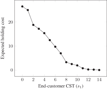
Figure 6.17 SSSPP trade‐off curve: expected cost vs. end‐customer CST.
The guaranteed‐service model is particularly adept at deciding whether stages should operate in push or pull mode since it tends to generate solutions in which only a subset of the stages hold inventory. For instance, suppose we reduce the CST of the Imager assembly stage in Figure 6.15 so that Ship to final assembly holds less inventory and Imager assembly begins to hold some. This means increasing the NLT at Imager assembly and decreasing it at Ship to final assembly. Since the safety stock is a concave function of the NLT, increasing the NLT at Imager assembly has a larger impact on the objective function than does decreasing the NLT at Ship to Final assembly from 10. This makes it unlikely to be a cost‐effective change, unless the holding cost is much cheaper at Imager assembly.
In contrast, the objective of the stochastic‐service model is a convex function of the base‐stock level of each stage (see Section 6.2.2), encouraging the inventory to be more evenly distributed throughout the system.
Although the stochastic‐ and guaranteed‐service models describe the system in different ways and produce different sets of base‐stock levels, it is important to note that these are modeling differences rather than operational ones. That is, once we set the base‐stock levels, the system operates the same, whether those base‐stock levels were set using the stochastic‐ or guaranteed‐service approach. In the guaranteed‐service model, there is no need to impose an operational rule requiring orders to be shipped within S periods; the CSTs will automatically be satisfied as a result of the base‐stock levels and the demand bound. (See Problem 6.12.) And in the stochastic‐service model, there is no need to require demands to be satisfied from stock whenever possible; that, too, will happen as a result of the base‐stock levels.
Which model we choose depends on how accurately each one models the particular features of the real‐world system and how tractable each one is. In our experience, stochastic‐service models tend to be a more natural way to describe most real‐world supply chains (since managers are more accustomed to thinking in terms of inventory levels than in terms of CSTs). On the other hand, guaranteed‐service models are typically much more tractable and have therefore been implemented in more commercial software packages for multiechelon inventory optimization than stochastic‐service models have.
PROBLEMS
- 6.1 (Exact Algorithm for Serial Systems) Using the exact algorithm for serial systems with stochastic service in Section 6.2.2, find optimal base‐stock levels for the following instance:
 ,
,  ,
,  ,
,  , and the demand per unit time is distributed
  . Report both echelon and local base‐stock levels (
 and
and  ).
). - 6.2 (Shang–Song Heuristic) Using the Shang–Song heuristic discussed in Section 6.2.3, find near‐optimal base‐stock levels for the following instance:
 ,
,  ,
,  ,
,  , and
, and  .
.- Assume the demand per unit time is normally distributed with a mean of 64 and a standard deviation of 8.
- Assume the demand per unit time has a Poisson distribution with
 .
. Report both echelon and local base‐stock levels (
 and
and  ).
).
- 6.3 (Comparison of Exact and Heuristic Approaches) Find optimal and near‐optimal base‐stock levels for the following serial system using both the exact approach from Section 6.2.2 and the Shang–Song heuristic from Section 6.2.3:
 ,
,  ,
,  ,
,  for all j, and the demand per unit time is distributed
  . Report the echelon base‐stock levels and the expected cost of each solution.
 - 6.4 (Proof of Proposition 6.1) ProveProposition 6.1.
- 6.5 (Equivalence of Local‐ and Echelon‐Based Total Costs) Prove that
 in 6.8 equals
  in 6.9.
 - 6.6 (Proof of “All‐or‐Nothing” Theorem) ProveTheorem 6.4.
Note: You may use the fact that there exists an optimal solution in which, for all i, either
 or
or  .
. - 6.7 (Safety Stock for Ceramic Plates) A manufacturer of ceramic plates and other tableware divides the manufacturing process into three major steps: forming, firing, and glazing. In the first step, the plates are formed out of clay; in the second, the plates are heated in a kiln, and in the third, the plates are painted. Forming and firing each take 1 day, while glazing takes 2 days. Clay is procured from an external vendor, which delivers orders exactly 1 day after they are placed. The daily demand for plates, as measured in cases, is distributed
 . The company promises its customers that finished (i.e., glazed) plates will always be on‐hand provided that the demand on a given day is no more than 4 standard deviations above its mean. (That is,
  and
and  .) Inventory may be held at any stage of the process. The holding cost of one case of plates (or its precursor products) is $2 per day for plates that have been formed but not fired, $3 for plates that have been fired but not glazed, and $4 for glazed plates. Find the optimal CST, base‐stock level, and safety‐stock level at each stage, as well as the optimal expected cost per day.
 - 6.8 (Implementing Serial SSSPP DP) The file
serial10.xlsxcontains the holding costs and processing times for a 10‐stage serial system. The demand per period is distributed . Use
. Use  in the demand bound. There is an inbound service time of 7 periods at stage 10, and stage 1 has a CST of 3 to the customer. Implement the DP algorithm from Section 6.3.4 and use it to find the optimal CST, base‐stock level, and safety‐stock level at each stage, as well as the optimal expected cost per period.
 - 6.9 (Safety Stock for Baseball Hats)
Figure 6.18 depicts the supply chain for a firm that manufactures baseball hats for college baseball fans. There are two end products. Product 1 is a Lehigh University hat, for which the firm sees a daily demand that is normally distributed with a mean of 22.0 cases and a standard deviation of 4.1 cases. Product 2 is a Lafayette College hat, whose demand is also normally distributed, with a mean of 15.3 cases and a standard deviation of 6.2 cases.
Stage 3 represents assembling the hats from two subassemblies: the cap (the part that sits on your head) and the visor (the part that sticks out in front). This generic product is then differentiated at stages 1 and 2 by dyeing the fabric and embroidering the team logos. Stage 4 represents the visor subassembly, while stage 5 represents sewing the cap subassembly out of fabric; the fabric is represented by stage 6.
Figure 6.18 indicates the processing time below each stage and, above it, the value of one case's worth of the product. The firm is committed to providing a CST of 3 days to its customers (such as college bookstores). It has also set CSTs for the upstream stages, which are indicated on the links in the figure, but you suspect that these are not the optimal CSTs.
- Calculate the base‐stock level and safety‐stock level required at each stage for the solution in the figure, as well as the total expected holding cost. Assume that demands are truncated 4 standard deviations above their means; i.e.,
 in 6.33. Also assume that holding costs are calculated as 20% of the product value, per year. (Make sure to translate into days.)
 - Develop a solution to the SSSPP that still gives CSTs of 3 days to the end customers but is cheaper than the solution depicted in Figure 6.18. Your solution does not need to be optimal, only better than the one in Figure 6.18. For each stage, report the CST, base‐stock level, and safety‐stock level, as well as the total expected holding cost per period for the whole system.

Figure 6.18 Baseball‐hat supply chain for Problem 6.9.
- Calculate the base‐stock level and safety‐stock level required at each stage for the solution in the figure, as well as the total expected holding cost. Assume that demands are truncated 4 standard deviations above their means; i.e.,
- 6.10 (Implementing Tree SSSPP DP) Implement Algorithm 6.2 and use it to find the optimal solution for the instance introduced in Problem 6.9. Report the optimal CST, base‐stock level, and safety‐stock level at each stage, as well as the optimal expected cost per period.
- 6.11 (Two‐Stage SSSPP) Consider a two‐stage serial supply chain with guaranteed service as defined in Section 6.3.4. Assume that
 . The inbound CST to stage 2,
  , is a constant, as is the outbound CST from stage 1,
  . Therefore, the only decision variable is
  . For simplicity, assume that
  . Then the objective function is given by
- Prove that, in the optimal solution to the SSSPP for the two‐stage supply chain defined above:
- Stage 1 holds safety stock if and only if
 .
. - If stage 1 holds safety stock, then stage 2 also holds safety stock if and only if

- Stage 1 holds safety stock if and only if
- Now consider an N‐stage serial supply chain, with
 and
and  constants, as usual. Assume that
  . Prove that if then stages
 hold no safety stock.
- Prove that, in the optimal solution to the SSSPP for the two‐stage supply chain defined above:
- 6.12 (CSTs are Satisfied) Simulate a single‐stage system under the guaranteed‐service model in a programming language or spreadsheet program of your choice. Assume
 ,
,  , and
, and  . Assume the demand per period is distributed as
  and use
  to truncate the demand. Use the appropriate base‐stock level y for these settings and assume the system begins period 1 with y units on hand. Assume that demands are satisfied first‐come, first‐served. Simulate the system for at least 1000 periods and verify that, as claimed in Section 6.4, the CST is always satisfied, even though your simulation does not contain explicit logic to ensure it.
 Hint: Include columns or variables that keep track of the number of unsatisfied demands that were placed 0, 1, 2, 3, and 4 or more periods ago.
- 6.13 (Limits of
 Function) In the exact algorithm for serial systems described in Section 6.2.2, prove that, for all
  : (6.53)
 (6.54)
where
 if
if  . What types of functions are these (quadratic, linear, concave, etc.)?
 - 6.14 (Proof of
6.13) In this problem you will prove 6.13. Throughout this problem, you may use any of the results up until 6.12, but nothing that comes later.
- Prove that

- Use part (a) to prove that

- Prove that
- 6.15 (Approximate Two‐Stage SSM Model) Consider a 2‐stage serial system following an echelon base‐stock policy under the SSM model. The costs, demand rate, and lead times are as given in Section 6.2.1. Assume the demand per unit time is distributed as
 , so the lead‐time demand for stage j has a mean of
  and a standard deviation of
  .
. In this problem, you will develop an approximate method for computing the cost of a given echelon base‐stock policy. This method is much easier to implement than the Clark–Scarf recursion in Theorem 6.2.
From 6.9, the expected cost for a given echelon base‐stock policy
 can be written
This expression has three random variables; you'll use exact expressions for the expectations of the first two and develop an approximation for the third.
From 6.30,
At stage 2,
 since stage 2's supplier never has stockouts. Therefore, from 6.16,(6.56)
 (6.57)
- Prove that (6.58)

where
 is the standard normal loss function. You may assume
  .
. - From 6.16,
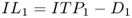 . To calculate
  exactly, therefore, we need to use the distribution of
  . Unfortunately, this distribution is fairly complicated. The approximation we are proposing instead is to replace the stochastic
  with its mean,
  . (We are not suggesting this is a very good approximation. In general, replacing a random variable with its mean can lead to significant inaccuracy. But it makes the problem more tractable, so we will try it.)
 Prove that, under this approximation,
(6.59)
- Do you think the approximation in part (b) will underestimate or overestimate
 ? Explain your answer in one or two sentences.
- Prove that
- 6.16 (Implementing Approximate Two‐Stage SSM Model) Implement the approximation from Problem 6.15 in MATLAB to compute the expected cost using the optimal
 and a given value for
  .
. (Hint: To double‐check that your calculations are correct, we'll tell you the following: If
 ,
,  ,
,  ,
,  ,
,  ,
,  ,
,  , then
  .)
.)- Compute the optimal
 for a system with
  ,
,  ,
,  ,
,  ,
,  ,
,  , and
, and  . Use 6.55 to find
  , then find
  in MATLAB using a method of your choosing: trial and error; MATLAB's
 fminuncfunction; etc. Report ,
,  , and
, and  . Include a printout of all MATLAB code, including a transcript of the session in which you found
  .
. - Compute values for the following quantities assuming
 is set to the optimal values from part (a). (Hint: You should not have to evaluate any more integrals.)
 - The expected on‐hand inventory at stage 1,
 .
. - The expected backorders at stage 1,
 .
. - The expected inventory level at stage 1,
 .
. - The expected local on‐hand inventory at stage 2,
 .
. - The expected local backorders at stage 2,
 .
. - The expected echelon inventory level at stage 2,
 .
. - The expected number of units in transit from stage 2 to stage 1,
 .
. - The expected holding, stockout, and total costs per period.
- The expected on‐hand inventory at stage 1,
- Compute the optimal