
Chapter 16
Cost-Benefit Analysis Using Data-Driven Costs
In Chapter 15, we were introduced to cost-benefit analysis and misclassification costs. Our goal in this chapter is to derive a methodology whereby the data itself teaches us what the misclassification costs should be; that is, cost-benefit analysis using data-driven misclassification costs. Before we can perform that, however, we must turn to a more systematic treatment of misclassification costs and cost-benefit tables, deriving the following three important results regarding misclassification costs and cost-benefit tables1
:
- Decision invariance under row adjustment
- Positive classification criterion
- Decision invariance under scaling.
16.1 Decision Invariance Under Row Adjustment
For a binary classifier, define ![]() to be the confidence (to be defined later) of the model for classifying a data record as i = 0 or i = 1. For example,
to be the confidence (to be defined later) of the model for classifying a data record as i = 0 or i = 1. For example, ![]() represents the confidence that a given classification algorithm has in classifying a record as positive (1), given the data.
represents the confidence that a given classification algorithm has in classifying a record as positive (1), given the data. ![]() is also called the posterior probability of a given classification. By way of contrast,
is also called the posterior probability of a given classification. By way of contrast, ![]() would represent the prior probability of a given classification; that is, the proportion of 1's or 0's in the training data set. Also, let
would represent the prior probability of a given classification; that is, the proportion of 1's or 0's in the training data set. Also, let ![]() , and
, and ![]() represent the cost of a true negative, a false positive, a false negative, and a true positive, respectively, for the cost matrix shown in Table 16.1.
represent the cost of a true negative, a false positive, a false negative, and a true positive, respectively, for the cost matrix shown in Table 16.1.
Table 16.1 Cost matrix for binary classifier
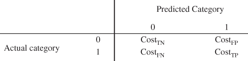 |
Then, the expected cost of a positive or negative classification may be written as follows:
For a positive classification, this represents the weighted average of the costs in the positive predicted column, weighted by the confidence for classifying the records as negative and positive, respectively. It is similar for a negative classification. The minimum expected cost principle is then applied, as described here.
Thus, a data record will be classified as positive if and only if the expected cost of the positive classification is no greater than the expected cost of the negative classification. That is, we will make a positive classification if and only if:
That is, if and only if:
Now, suppose we subtract a constant a from each cell in the top row of the cost matrix (Table 16.1), and we subtract a constant b from each cell in the bottom row. Then equation (16.1) becomes
which simplifies to equation (16.1). Thus, we have Result 1.
16.2 Positive Classification Criterion
We use Result 1 to develop a criterion for making positive classification decisions, as follows. First, subtract ![]() from each cell in the top row of the cost matrix, and subtract
from each cell in the top row of the cost matrix, and subtract ![]() from each cell in the bottom row of the cost matrix. This gives us the adjusted cost matrix shown in Table 16.2.
from each cell in the bottom row of the cost matrix. This gives us the adjusted cost matrix shown in Table 16.2.
Table 16.2 Adjusted cost matrix
 |
Result 1 means that we can always adjust the costs in our cost matrix so that the two cells representing correct decisions have zero cost. Thus, the adjusted costs are

Rewriting equation (16.1), we will then make a positive classification if and only if:
As ![]() , we can re-express equation (16.2) as
, we can re-express equation (16.2) as
which, after some algebraic modifications, becomes:
This leads us to Result 2.
16.3 Demonstration Of The Positive Classification Criterion
For C5.0 models, the model's confidence in making a positive or negative classification is given as
The model's positive confidence PC is then calculated as
We demonstrate the positive classification criterion using the Adult2_training data set and the Adult2_test data set, as follows. First, three C5.0 classification models are trained on the training data set:
- Model A, with no misclassification costs. Here,
 and
and  , so that
  and the positive confidence threshold is
  . Thus, Model A should make positive classifications when
  .
. - Model B, with
 , and
, and  . Here,
  and the positive confidence threshold is
  . Thus, Model B should make positive classifications when
  .
. - Model C, with
 , and
, and  . Here,
  and the positive confidence threshold is
 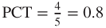 . Thus, Model C should make positive classifications when
  .
.
Each model is evaluated on the test data set. For each record for each model, the model's positive confidence PC is calculated. Then, for each model, a histogram of the values of PC is constructed, with an overlay of the target classification. These histograms are shown in Figures 16.1a–c for Models A, B, and C, respectively. Note that, as expected:
- For Model A, the model makes positive classifications, whenever
 .
. - For Model B, the model makes positive classifications, whenever
 .
. - For Model C, the model makes positive classifications, whenever
 .
.

Figure 16.1 (a) Model A: Positive classification when  . (b) Model B: Positive classification when
  . (c) Model C: Positive classification when
  .
.
16.4 Constructing The Cost Matrix
Suppose that our client is a retailer seeking to maximize revenue from a direct marketing mailing of coupons to likely customers for an upcoming sale. A positive response represents a customer who will shop the sale and spend money. A negative response represents a customer who will not shop the sale and spend money. Suppose that mailing a coupon to a customer costs $2, and that previous experience suggests that those who shopped similar sales spent an average of $25.
We calculate the costs for this example as follows:
- True Negative. This represents a customer who would not have responded to the mailing being correctly classified as not responding to the mailing. The actual cost incurred for this customer is zero, because no mailing was made. Therefore, the direct cost for this decision is $0.
- True Positive. This represents a customer who would respond to the mailing being correctly classified as responding to the mailing. The mailing cost is $2, while the revenue is $25, so that the direct cost for this customer is $2 − $25 = −$23.
- False Negative. This represents a customer who would respond positively to the mailing, but was not given the chance because he or she was incorrectly classified as not responding to the mailing, and so was not sent a coupon. The direct cost is $0.
- False Positive. This represents a customer who would not shop the sale being incorrectly classified as responding positively to the mailing. For this customer, the direct cost is the mailing expense, $2.
These costs are summarized in Table 16.3.
Table 16.3 Cost matrix for the retailer example
 |
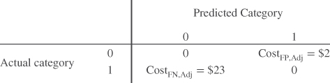
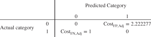
Then, by Result 1 (decision invariance under row adjustment), we derive the adjusted cost matrix in Table 16.4 by subtracting ![]() from each cell in the bottom row. Note that the costs representing the two correct classifications equal zero. Software packages such as IBM/SPSS Modeler require the cost matrix to be in a form where there are zero costs for the correct decisions, such as in Table 16.4.
from each cell in the bottom row. Note that the costs representing the two correct classifications equal zero. Software packages such as IBM/SPSS Modeler require the cost matrix to be in a form where there are zero costs for the correct decisions, such as in Table 16.4.
Table 16.4 Adjusted cost matrix for the retailer example
 |
16.5 Decision Invariance Under Scaling
Now, Result 2 states that we will make a positive classification when a model's PC is not less than the following:
Examining equation (16.3), we can see that the new adjusted cost matrices in Tables 16.5 and 16.6 are equivalent to the adjusted cost matrix in Table 16.4 for the purposes of rendering a classification decision. If it is important, say for interpretation purposes, for one of the adjusted costs to be expressed as a unit (e.g., $1), then this can be done – for either adjusted cost – by dividing through by the appropriate adjusted cost. For example, we can tell our client that, for every dollar that a false positive costs us, a false negative costs us $11.50 (Table 16.5); or conversely, for every dollar that a false negative costs us, a false positive costs us only eight cents (Table 16.6).
Table 16.5 Adjusted cost matrix, where the false positive adjusted cost equals 1
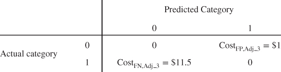 |
Table 16.6 Adjusted cost matrix, where the false negative adjusted cost equals 1
 |
What we are doing here is scaling (dividing) by one of the adjusted costs; hence, we have Result 3.
For example, the pairs of adjusted costs in Table 16.7 are equivalent for the purposes of rendering a classification decision:
Table 16.7 Pairs of equivalent adjusted costs
| Adjusted Cost Matrix | Adjusted False Positive Cost | Adjusted False Negative Cost |
| Original | ||
| Scaled by |
||
| Scaled by |
Important note: When calculating the total cost of a classification model, or when comparing the total cost of a set of models, the analyst should use the original unadjusted cost matrix as shown in Table 16.3, and without applying any matrix row adjustment or scaling. The row adjustment and scaling leads to equivalent classification decisions, but it changes the reported costs of the final model. Therefore, use the unadjusted cost matrix when calculating the total cost of a classification model.
16.6 Direct Costs and Opportunity Costs
Direct cost represents the actual expense of the class chosen by the classification model, while direct gain is the actual revenue obtained by choosing that class. Our cost matrix above was built using direct costs only. However, opportunity cost represents the lost benefit of the class that was not chosen by the classification model. Opportunity gain represents the unincurred cost of the class that was not chosen by the classification model. We illustrate how to combine direct costs and opportunity costs into total costs, which can then be used in a cost-benefit analysis, using the following example. For example, for the false negative situation, the opportunity gain is $2, in that the client saved the cost of the coupon, but the opportunity cost is $25, in that the client did not receive the benefit of the $25 in revenue this customer would have spent. So, the opportunity cost is $25 − $2 = $23. Why then, do not we use opportunity costs when constructing the cost matrix? Because doing so would double count the costs. For example, a switch of a single customer from a false negative to a true positive would result in an decrease in model cost of $46 if we counted both the false negative opportunity cost and the true positive direct cost, which is twice as much as a single customer spends, on average.2
16.7 Case Study: Cost-Benefit Analysis Using Data-Driven Misclassification Costs
Many of the concepts presented in this chapter are now brought together in the following case study application of cost-benefit analysis using data-driven misclassification costs. In this era of big data, businesses should leverage the information in their existing databases in order to help uncover the optimal predictive models. In other words, as an alternative to assigning misclassification costs because “these cost values seem right to our consultant” or “that is how we have always modeled them,” we would instead be well advised to listen to the data, and learn from the data itself what the misclassification costs should be. The following case study illustrates this process.
The Loans data set represents a set of bank loan applications for a 3-year term. Predictors include debt-to-income ratio, request amount, and FICO score. The target variable is approval; that is, whether or not the loan application is approved, based on the predictor information. The interest represents a flat rate of 15% times the request amount, times 3 years, and should not be used to build prediction models. The bank would like to maximize its revenue by funding the loan applications that are likely to be repaid, and not funding those loans that will default. (We make the simplifying assumption that all who are approved for the loan actually take the loan.)
Our strategy for deriving and applying data-driven misclassification costs is as follows.
Table 16.8 Adjusted cost matrix for the bank loan case study
 |
Note that our misclassification costs are data-driven, meaning that the data set itself is providing all of the information needed to assign the values of the misclassification costs. Using the Loans_training data set, we find that the mean amount requested is $13,427, and the mean amount of loan interest is $6042. A positive decision represents loan approval. We make a set of simplifying assumptions, to allow us to concentrate on the process at hand, as follows.
We proceed to develop the cost matrix, as follows.
- True Negative. This represents an applicant who would not have been able to repay the loan (i.e., defaulted) being correctly classified for non-approval. The cost incurred for this applicant is $0, because no loan was proffered, no interest was accrued, and no principal was lost.
- True Positive. This represents an applicant who would reliably repay the loan being correctly classified for loan approval. The bank stands to make $6042 (the mean amount of loan interest) from customers such as this. So the cost for this applicant is −$6042.
- False Negative. This represents an applicant who would have reliably paid off the loan, but was not given the chance because he or she was incorrectly classified for non-approval. The cost incurred for this applicant is $0, because no loan was proffered, no interest was accrued, and no principal was lost.
- False Positive. This represents an applicant who will default being incorrectly classified for loan approval. This is a very costly error for the bank, directly costing the bank the mean loan amount requested, $13,427.
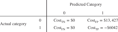
We summarize the costs in Table 16.9.
Table 16.9 Matrix of direct costs for the bank loan case study
 |
Table 16.9 will be used to calculate the total cost of any classification models built using these misclassification costs.
We adjust the cost matrix in Table 16.9 to make it conducive to the software, by subtracting ![]() from the bottom row, giving us the adjusted cost matrix in Table 16.8.
from the bottom row, giving us the adjusted cost matrix in Table 16.8.
For simplicity, we apply Result 3, scaling each of the non-zero costs by ![]() , to arrive at the cost matrix shown in Table 16.10.
, to arrive at the cost matrix shown in Table 16.10.
Table 16.10 Simplified cost matrix for the bank loan case study
 |
Using the Loans_training data set, two CART models are constructed:
- Model 1: The naïve CART model with no misclassification costs, used by the bank until now.
- Model 2: The CART model with misclassification costs specified in Table 16.10.
These models are then evaluated using the Loans_test data set. The resulting contingency tables for Model 1 and Model 2 are shown in Tables 16.11 and 16.12, respectively. These counts were evaluated using the matrix of total costs in Table 16.9.
Table 16.11 Contingency table for Model 1 with no misclassification costs
 |
Table 16.12 Contingency table for Model 2, with data-driven misclassification costs
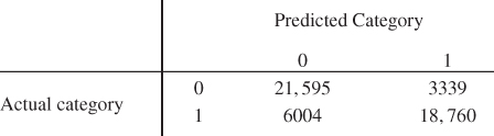 |
Table 16.13 contains the evaluation measures for Models 1 and 2, with the better performing model's results in bold. Note that Model 1 performs better with the following measures: accuracy, overall error rate, sensitivity, false positive rate, proportion of true negatives, and proportion of false negatives. Model 2 performs better with respect to specificity, false negative rate, proportion of true positives, and proportion of false positives. Recall that, for the bank, the false positive error is the more costly mistake. Thus, Model 2, with its heavier penalty for making the false positive error, delivers a lower proportion of false positives (0.1511 vs 0.2191). But most importantly, Model 2 delivers where it counts: in the bottom line. The overall model cost is ![]() for Model 1 and
for Model 1 and ![]() for Model 2, meaning that the increase in revenue for the model using misclassification costs compared to the model not using misclassification costs is
for Model 2, meaning that the increase in revenue for the model using misclassification costs compared to the model not using misclassification costs is
Table 16.13 Evaluation measures. Model 2, with data-driven misclassification costs, has increased revenue by nearly $15 million (better performance in bold)
| CART Model | ||
| Evaluation Measure | Model 1: Without Misclassification Costs | Model 2: With Misclassification Costs |
| Accuracy | 0.8432 | 0.8120 |
| Overall error rate | 0.1568 | 0.1880 |
| Sensitivity | 0.9527 | 0.7576 |
| False positive rate | 0.0473 | 0.2424 |
| Specificity | 0.7345 | 0.8661 |
| False negative rate | 0.2655 | 0.1339 |
| Proportion of true positives | 0.7809 | 0.8489 |
| Proportion of false positives | 0.2191 | 0.1511 |
| Proportion of true negatives | 0.9399 | 0.7825 |
| Proportion of false negatives | 0.0601 | 0.2175 |
| Overall model cost | ||
| Revenue per applicant | ||
That is, the simple step of applying data-driven misclassification costs has led to an increase in revenue of nearly $15 million. This represents a per-applicant increase in revenues of $1379 − $1080 = $299.
16.8 Rebalancing as a Surrogate for Misclassification Costs
Not all algorithms have an explicit method for applying misclassification costs. For example, the IBM/SPSS Modeler implementation of neural network modeling does not allow for misclassification costs. Fortunately, data analysts may use rebalancing as a surrogate for misclassification costs. Rebalancing refers to the practice of oversampling either the positive or negative responses, in order to mirror the effects of misclassification costs. The formula for the rebalancing, due to Elkan,3 is as follows.
For the bank loan case study, we have ![]() , so that our resampling ratio is
, so that our resampling ratio is ![]() . We therefore multiply the number of records with negative responses (Approval = F) in the training data set by 2.22. This is accomplished by resampling the records with negative responses with replacement.
. We therefore multiply the number of records with negative responses (Approval = F) in the training data set by 2.22. This is accomplished by resampling the records with negative responses with replacement.
We then provide the following four network models:
- Model 3: The naïve neural network model, constructed on a training set with no rebalancing.
- Model 4: A neural network model constructed on a training set with a = 2.0 times as many negative records as positive records.
- Model 5: The neural network model constructed on a training set with a = 2.22 times as many negative records as positive records.
- Model 6: A neural network model constructed on a training set with a = 2.5 times as many negative records as positive records.
Table 16.14 contains the counts of positive and negative responses in the training data set, along with the achieved resampling ratio for each of Models 3–6. Note that the higher counts for the negative responses were accomplished through resampling with replacement.
Table 16.14 Counts of negative and positive responses, and achieved resampling ratios
| Negative Responses | Positive Responses | Desired Resampling Ratio | Achieved Resampling Ratio | |
| Model 3 | 75,066 | 75,236 | N/A | N/A |
| Model 4 | 150,132 | 75,236 | 2.0 | |
| Model 5 | 166,932 | 75,236 | 2.22 | |
| Model 6 | 187,789 | 75,236 | 2.5 |
The four models were then evaluated using the test data set. Table 16.15 contains the evaluation measures for these models.
Table 16.15 Evaluation measures for resampled models. The resampled neural network model with the data-driven resampling ratio, is the highest performing model of all (best performing model highlighted)
| CART Model | ||||
| Evaluation Measure | Model 3: None | Model 4: a = 2.0 | Model 5: a = 2.22 | Model 6: a = 2.5 |
| Accuracy | 0.8512 | 0.8361 | 0.8356 | 0.8348 |
| Overall error rate | 0.1488 | 0.1639 | 0.1644 | 0.1652 |
| Sensitivity | 0.9408 | 0.8432 | 0.8335 | 0.8476 |
| False positive rate | 0.0592 | 0.1568 | 0.1665 | 0.1526 |
| Specificity | 0.7622 | 0.8291 | 0.8376 | 0.8221 |
| False negative rate | 0.2378 | 0.1709 | 0.1624 | 0.1779 |
| Proportion of true positives | 0.7971 | 0.8305 | 0.8360 | 0.8256 |
| Proportion of false positives | 0.2029 | 0.1695 | 0.1640 | 0.1744 |
| Proportion of true negatives | 0.9284 | 0.8418 | 0.8351 | 0.8446 |
| Proportion of false negatives | 0.0716 | 0.1582 | 0.1649 | 0.1554 |
| Overall model cost | ||||
| Revenue per applicant | ||||
Note that Model 5, whose resampling ratio of 2.22 is data-driven, being entirely specified by the data-driven adjusted misclassification costs, is the highest performing model of all, with model cost of ![]() , and a per-applicant revenue of $1415. In fact, the neural network model with 2.22 rebalancing outperformed our previous best model, the CART model with misclassification costs, by
, and a per-applicant revenue of $1415. In fact, the neural network model with 2.22 rebalancing outperformed our previous best model, the CART model with misclassification costs, by
This $1.83 million may have been lost had the bank's data analyst not had recourse to the technique of using rebalancing as a surrogate for misclassification costs.
Why does rebalancing work? Take the case where ![]() . Here, the false positive is the more expensive error. The only way a false positive error can arise is if the response should be negative. Rebalancing provides the algorithm with a greater number of records with a negative response, so that the algorithm can have a richer set of examples from which to learn about records with negative responses. This preponderance of information about records with negative responses is taken into account by the algorithm, just as if the weight of these records was greater. This diminishes the propensity of the algorithm to classify a record as positive, and therefore decreases the proportion of false positives.
. Here, the false positive is the more expensive error. The only way a false positive error can arise is if the response should be negative. Rebalancing provides the algorithm with a greater number of records with a negative response, so that the algorithm can have a richer set of examples from which to learn about records with negative responses. This preponderance of information about records with negative responses is taken into account by the algorithm, just as if the weight of these records was greater. This diminishes the propensity of the algorithm to classify a record as positive, and therefore decreases the proportion of false positives.
For example, suppose we have a decision tree algorithm that defined confidence and PC as follows:
And suppose (for illustration) that this decision tree algorithm did not have a way to define the misclassification costs, ![]() . Consider Result 2, which states that a model will make a positive classification if and only if its positive confidence is greater than the positive confidence threshold; that is, if and only if
. Consider Result 2, which states that a model will make a positive classification if and only if its positive confidence is greater than the positive confidence threshold; that is, if and only if
where
The algorithm does not have recourse to the misclassification costs on the right-hand side of the inequality ![]()
. However, equivalent behavior may be obtained by manipulating the PC on the left-hand side. Because ![]() , we add extra negative-response records, which has the effect of increasing the typical number of records in each leaf across the tree, which, because the new records are negative, typically reduces the PC. Thus, on average, it becomes more difficult for the algorithm to make positive predictions, and therefore fewer false positive errors will be made.
, we add extra negative-response records, which has the effect of increasing the typical number of records in each leaf across the tree, which, because the new records are negative, typically reduces the PC. Thus, on average, it becomes more difficult for the algorithm to make positive predictions, and therefore fewer false positive errors will be made.
R References
- 1. Kuhn M, Weston S, Coulter N. 2013. C code for C5.0 by R. Quinlan. C50: C5.0 decision trees and rule-based models. R package version 0.1.0-15. http://CRAN.R-project.org/package=C50.
- 2. R Core Team. R: A Language and Environment for Statistical Computing. Vienna, Austria: R Foundation for Statistical Computing; 2012. ISBN: 3-900051-07-0, http://www.R-project.org/.
Exercises
For Exercises 1–8, state what you would expect to happen to the indicated classification evaluation measure, if we increase the false negative misclassification cost, while not increasing the false positive cost. Explain your reasoning.
1. Sensitivity.
2. False positive rate.
3. Specificity.
4. False negative rate.
5. Proportion of true positives.
6. Proportion of false positives.
7. Proportion of true negatives
8. Proportion of false negatives.
9. True or false: The overall error rate is always the best indicator of a good model.
10. Describe what is meant by the minimum expected cost principle.
11. Explain decision invariance under row adjustment.
12. True or false: We can always adjust the costs in our cost matrix so that the two cells representing correct decisions have zero cost.
13. What is the difference between confidence and positive confidence?
14. What is the adjusted false positive cost? The adjusted false negative cost?
15. What is the positive confidence threshold?
16. Explain the positive classification criterion.
17. Clearly explain how Figure 16.1 demonstrates the positive classification criterion for a C5.0 binary classifier.
18. Explain what is meant by decision invariance under scaling.
19. How might Result 3 be of use to an analyst making a presentation to a client?
20. What are direct costs? Opportunity costs? Why should we not include both when constructing our cost matrix?
21. What do we mean when we say that the misclassification costs in the case study are data-driven?
22. In the case study, explain why Model 1 has better sensitivity, lower proportion of false negatives, and lower overall error rate. Then explain why Model 2 is better.
23. Why might we need rebalancing as a surrogate for misclassification costs?
24. Explain how we do such rebalancing when the adjusted false positive cost is greater than the adjusted false negative cost.
25. What does it mean to say that the resampling ratio is data-driven?
26. Why does rebalancing work as a surrogate for misclassification costs?
Use the following information for Exercises 27–44.
Suppose that our client is a retailer seeking to maximize revenue from a direct marketing mailing of coupons to likely customers for an upcoming sale. A positive response represents a customer who will shop the sale and spend money. A negative response represents a customer who will not shop the sale and spend money. Suppose that mailing a coupon to a customer costs $5, and that previous experience suggests that those who shopped similar sales spent an average of $100.
27. Explain why (i) misclassification costs are needed in this scenario, and (ii) the overall error rate is not the best measure of a good model.
28. Construct the cost matrix. Provide rationales for each cost.
29. Use Result 1 to construct the adjusted cost matrix. Interpret the adjusted costs.
30. Calculate the positive confidence threshold. Use Result 2 to state when the model will make a positive classification.
31. Use Result 3 to readjust the adjusted misclassification costs, so that the readjusted false positive cost is $1. Interpret the readjusted false positive and false negative costs.
32. Use Result 3 to readjust the adjusted misclassification costs, so that the readjusted false negative cost is $1. Interpret the readjusted false positive and false negative costs.
For Exercises 33–42, consider two classification models: Model 1 is a naïve model with no misclassification costs, and Model 2 uses the cost matrix you constructed earlier. Which model do you expect to perform better according to the following measures, and why?
33. Sensitivity.
34. False positive rate.
35. Specificity.
36. False negative rate.
37. Proportion of true positives.
38. Proportion of false positives.
39. Proportion of true negatives.
40. Proportion of false negatives.
41. Model cost.
42. Revenue per customer.
43. Suppose the classification algorithm of choice had no method of applying misclassification costs.
- What would be the resampling ratio for using rebalancing as a surrogate for misclassification costs?
- How should the training set be rebalanced?
44. Why don't we rebalance the test data set?
Hands-On Exercises
Use the Churn data set for Exercises 45–52. A positive response represents a churner (customer who will leave the company's service). A negative response represents a non-churner. Suppose that intervening with a customer in danger of churning costs $100, and that a customer who churns represents $2000 in lost revenue. Now, suppose the company's intervention strategy is useless, and that everyone the company intervenes with to stop churning will churn anyway.
45. Construct the cost matrix. Provide rationales for each cost.
46. Partition the Churn data set into a training data set and a test data set.
47. Using the training set, develop a CART model for predicting Churn. Do not use misclassification costs. Call this Model 1.
48. Using the training set, and the cost matrix, develop a CART model for predicting Churn. Call this Model 2.
49. Construct a table of evaluation measures for the two models, similarly to Table 16.13.
50. Report the increase or decrease in revenue, and the percentage increase or decrease in revenue per customer, obtained from using Model 2.
51. Next, assume the company's intervention strategy is perfect, and that everyone the company intervenes with to stop churning will not churn. Redo Exercises 45–50 under this assumption.
52. Finally, assume that 50% of those customers who are in danger of churning, and with whom the company intervenes, will stay with the company, and 50% will churn anyway. Redo Exercises 45–50 under this assumption.