3.3 Jeffreys’ rule

3.3.1 Fisher’s information

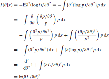
In Section 2.1 on the nature of Bayesian inference, the log-likelihood function was defined as

In this section, we shall sometimes write l for , L for and p for the probability density function . The fact that the likelihood can be multiplied by any constant implies that the log-likelihood contains an arbitrary additive constant.

An important concept in classical statistics which arises, for example, in connection with the Cramèr-Rao bound for the variance of an unbiased estimator, is that of the information provided by an experiment which was defined by Fisher (1925a) as

the expectation being taken over all possible values of x for fixed θ. It is important to note that the information depends on the distribution of the data rather than on any particular value of it, so that if we carry out an experiment and observe, for example, that , then the information is no different from the information if ; basically it is to do with what can be expected from an experiment before rather than after it has been performed. It may be helpful to note that strictly speaking it should be denoted

Because the log-likelihood differs from by a constant, all their derivatives are equal, and we can equally well define the information by

It is useful to prove two lemmas. In talking about these, you may find it useful to use a terminology frequently employed by classical statisticians. The first derivative of the log-likelihood is sometimes called the score; see Lindgren (1993, Section 4.5.4).

Lemma 3.1

.

Proof. From the definition

since in any reasonable case it makes no difference whether differentiation with respect to θ is carried out inside or outside the integral with respect to x.

Lemma 3.2

Proof. Again differentiating under the integral sign

as required.

3.3.2 The information from several observations

If we have n independent observations , then the probability densities multiply, so the log-likelihoods add. Consequently, if we define

then by linearity of expectation

where x is any one of the xi. This accords with the intuitive idea that n times as many observations should give us n times as much information about the value of an unknown parameter.

3.3.3 Jeffreys’ prior

In a Bayesian context, the important thing to note is that if we transform the unknown parameter θ to then

Squaring and taking expectations over values of x (and noting that does not depend on x), it follows that

It follows from this that if a prior density

is used, then by the usual change-of-variable rule

It is because of this property that Jeffreys (1961, Section 3.10) suggested that the density

provided a suitable reference prior (the use of this prior is sometimes called Jeffreys’ rule). This rule has the valuable property that the prior is invariant in that, whatever scale we choose to measure the unknown parameter in, the same prior results when the scale is transformed to any particular scale. This seems a highly desirable property of a reference prior. In Jeffreys’ words, ‘any arbitrariness in the choice of parameters could make no difference to the results’.

3.3.4 Examples

Normal mean. For the normal mean with known variance, the log-likelihood is

so that

which does not depend on x, so that

implying that we should take a prior

which is the rule suggested earlier for a reference prior.

Normal variance. In the case of the normal variance

so that

Because , it follows that

implying that we should take a prior

which again is the rule suggested earlier for a reference prior.

Binomial parameter. In this case,

so that

Because , it follows that

implying that we should take a prior

that is , that is π has an arc-sine distribution, which is one of the rules suggested earlier as possible choices for the reference prior in this case.

3.3.5 Warning

While Jeffreys’ rule is suggestive, it cannot be applied blindly. Apart from anything else, the integral defining the information can diverge; it is easily seen to do so for the Cauchy distribution C, for example. It should be thought of as a guideline that is well worth considering, particularly if there is no other obvious way of finding a prior distribution. Generally speaking, it is less useful if there are more unknown parameters than one, although an outline of the generalization to that case is given later for reference.

3.3.6 Several unknown parameters

If there are several unknown parameters , the information provided by a single observation is defined as a matrix, the element in row i, column j, of which is

As in the one parameter case, if there are several observations , we get

If we transform to new parameters where , we see that if is the matrix the element in row i, column j of which is

then it is quite easy to see that

where JT is the transpose of , and hence that the determinant of the information matrix satisfies

Because is the Jacobian determinant, it follows that

provides an invariant prior for the multi-parameter case.

3.3.7 Example

Normal mean and variance both unknown. In this case, the log-likelihood is

so that

and hence

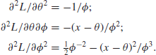
Because and , it follows that

and, so that

This implies that we should use the reference prior

It should be noted that this is not the same as the reference prior recommended earlier for use in this case, namely,

However, I would still prefer to use the prior recommended earlier. The invariance argument does not take into account the fact that in most such problems your judgement about the mean would not be affected by anything you were told about the variance or vice versa, and on those grounds it seems reasonable to take a prior which is the product of the reference priors for the mean and the variance separately.

The example underlines the fact that we have to be rather careful about the choice of a prior in multi-parameter cases. It is also worth mentioning that it is very often the case that when there are parameters which can be thought of as representing ‘location’ and ‘scale’, respectively, then it would usually be reasonable to think of these parameters as being independent a priori, just as suggested earlier in the normal case.