2.4 Dominant likelihoods

2.4.1 Improper priors

We recall from the previous section that, when we have several normal observations with a normal prior and the variances are known, the posterior for the mean is

where and are given by the appropriate formulae and that this approaches the standardized likelihood

insofar as is large compared with , although this result is only approximate unless is infinite. However, this would mean a prior density which, whatever θ0 were, would have to be uniform over the whole real line, and clearly could not be represented by any proper density function. It is basic to the concept of a probability density that it integrates to 1 so, for example,

cannot possibly represent a probability density whatever κ is, and in particular , which results from substituting into the normal density, cannot be a density. Nevertheless, we shall sometimes find it useful to extend the concept of a probability density to some cases like this where

which we shall call improper ‘densities’. The density can then be regarded as representing a normal density of infinite variance. Another example of an improper density we will have use for later on is

It turns out that sometimes when we take an improper prior density then it can combine with an ordinary likelihood to give a posterior which is proper. Thus, if we use the uniform distribution on the whole real line for some , it is easy to see that it combines with a normal likelihood to give the standardized likelihood as posterior; it follows that the dominant feature of the posterior is the likelihood. The best way to think of an improper density is as an approximation which is valid for some large range of values, but is not to be regarded as truly valid throughout its range. In the case of a physical constant which you are about to measure, you may be very unclear what its value is likely to be, which would suggest the use of a prior that was uniform or nearly so over a large range, but it seems unlikely that you would regard values in the region of, say, 10100 as being as likely as, say, values in the region of 10–100. But if you have a prior which is approximately uniform over some (possibly very long) interval and is never very large outside it, then the posterior is close to the standardized likelihood, and so to the posterior which would have resulted from taking an improper prior uniform over the whole real line. [It is possible to formalize the notion of an improper density as part of probability theory – for details, see Rényi (1970).]

2.4.2 Approximation of proper priors by improper priors

This result can be made more precise. The following theorem is proved by Lindley (1965, Section 5.2); the proof is omitted.

Theorem 2.1 A random sample of size n is taken from where is known. Suppose that there exist positive constants α, ε, M and c depending on x (small values of α and ε are of interest), such that in the interval defined by

where

the prior density of θ lies between ) and and outside it is bounded by Mc. Then the posterior density satisfies

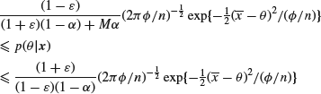
inside , and

outside it.

While we are not going to prove the theorem, it might be worth while to give some idea of the sorts of bounds which it implies. Anyone who has worked with the normal distribution is likely to remember that the 1% point is 2.58, that is that if then = 2.58, so that extends 2.58 standard deviations [] on each side of the sample mean . Suppose then that before you had obtained any data you believed all values in some interval to be equally likely, and that there were no values that you believed to be more than three times as probable as the values in this interval. If then it turns out when you get the data the range lies entirely in this interval, then you can apply the theorem with , , and M = 3, to deduce that within the true density lies within multiples and of the normal density. We can regard this theorem as demonstrating how robust the posterior is to changes in the prior. Similar results hold for distributions other than the normal.

It is often sensible to analyze scientific data on the assumption that the likelihood dominates the prior. There are several reasons for this, of which two important ones are as follows. Firstly, even if you and I both have strong prior beliefs about the value of some unknown quantity, we might not agree, and it seems sensible to use a neutral reference prior which is dominated by the likelihood and could be said to represent the views of someone who (unlike ourselves) had no strong beliefs a priori. The difficulties of public discourse in a world where different individuals have different prior beliefs constitute one reason why a few people have argued that, in the absence of agreed prior information, we should simply quote the likelihood function [see Edwards, 1992], but there are considerable difficulties in the way of this (see also Section 7.1 on ‘The Likelihood Principle’). Secondly, in many scientific contexts, we would not bother to carry out an experiment unless we thought it was going to increase our knowledge significantly, and if that is the case then the likelihood will presumably dominate the prior.