Chapter 3

External Antenna

The external antenna is the first member of the antenna family in the world of mobile phones. It appeared in the first commercial mobile phone, the Motorola DynaTAC 8000X, in 1983. External antennas were the only players in the mobile phone antenna market for more than 15 years. In the late 1990s, phones with internal antennas started to emerge. Candy-bar phones, also called single piece phones, with internal antennas rapidly expanded their market share in Europe; in the meantime external antennas in clam shell phones kept dominating the North America market for another five or more years. Eventually internal antennas took over the global antenna market.

The driving forces behind the fading of external antennas are both fashion and technical progress. Of the two, technical progress is the necessary condition. Even ten years after mobile phones came onto the market, there were just over one million users in the world at the end of 1993. In comparison, mobile subscriptions were more than three billion at the end of 2007. It is easy to imagine the user density was quite low after those limited users spread out. At that time, the most urgent issue was coverage. All mobile phone service providers wanted to expand their network coverage as much as possible with all the money they could spare. The coverage area of each base station depends on transmitting power, receivers' sensitivity, the path loss of electromagnetic wave, the antenna gain of base stations, and the antenna gain of mobile phones. The received signal power in dBm can be expressed by Equation (3.1):

(3.1)

where is the transmitter power in dBm. and are the transmitter and receiver antenna gains in dBi, relative to isotropic respectively. R is the distance between a base station and a mobile phone. C is a constant related to the frequency. α is the propagation attenuation factor, and normally it is a number between three and four in a city environment.

To get a phone to work properly, the received signal power must be higher than its sensitivity threshold. It is obvious that higher gain means larger coverage area. For example, assuming α equals three and the antenna gain of mobile phones is improved by 3 dB, the coverage area of the same base station will increase about 58%. When a phone is held by hand next to the head, the efficiency of a phone with an external whip antenna is likely to be 3 dB or more higher than one with an internal antenna. That made a huge difference when the mobile industry was still in its infancy.

There are two constraints on the mobile phone network planning. The first is how large an area each base station can cover. The second is how many users each station can support. In the beginning of the mobile phone's evolution, the primary challenge was how to design the whole system, including both base stations and mobile phones, to cover a huge area.

With the explosive adoption of mobile phones by the mass population, the atmosphere started to change. With more and more people enrolled into a mobile network, eventually the network reached a saturated status. All the available frequency resources or channels which could support users were exhausted. Now the second constraint, how to support more users, became the primary challenge. Fortunately, due to the cellular architecture that mobile networks adopted, there is a solution to this challenge. The total number of users a network can support depends on both the maximum capacity of each base station and the total number of base stations in the network. By adding more and more base stations to the network, the mobile service providers are able to keep up with the growth of mobile users. As a consequence, the distance between a mobile phone and the nearest base station is continuously shrinking. Shorter distance means less path loss, which in return reduces the requirement to improve antenna gain or antenna efficiency.

Compared to the United States, Europe has a much higher population density and started to shrink the cell size of each base station earlier. That partially explains why the European market was the first to successfully popularize the internal antenna. Actually the population density in Japan is even higher than Europe; however, candy-bar phones with internal antennas were not popularly accepted there. That can only be explained by fashion or cultural difference.

In the United States, one of the nationwide mobile providers, Nextel, merged with Sprint in 2003. Before the merger, Nextel ranked fifth or sixth in the US market, which was pretty close to the bottom of the list of nationwide providers. Nextel had a unique business model and some attractive services, such as Push-to-Talk (PTT) which is also marketed as “Walkie-Talkie from coast to coast.” This uniqueness gave Nextel the possibility of keeping its core customers and a considerable profit margin, but it also kept Nextel from expanding its customer base. Just before the merger, Nextel still had to cover the US with limited base stations. All the phones that Nextel carried had external antenna and most of them even had a whip in the antenna assembly.

To some, the external antenna is like a dinosaur and belongs to the last century. However, this is not necessarily true. With the adoption of MIMO (multiple-input and multiple-output) technology in handsets, external antennas might see their renaissance in the future. Another important reason for not writing off the external antenna is that there is a lot of mature and valuable knowledge in the designing of external antennas. Much of this knowledge can be applied to or referred to by designs of state-of-the-art internal monopole and ceramic antennas.

3.1 Stubby Antennas

There are mainly two kinds of external antennas: stubby antenna and whip-stubby antenna. A stubby antenna extrudes from a phone and does not have any movable parts. Earlier in the mobile phone's history, all stubby antennas were helix antennas made of copper wire or copper-coated steel wire (music wire). From the mechanical point of view, a helix antenna is the same as a spring coil and they can be cheaply made by the same machines and tools. When mass-produced, spring coils cost a few pennies a piece, so the helix antenna is a considerable cost-effective solution. A spring coil has a round cross-section, so a helix antenna normally possesses a column shape. That is why it has the name of “stubby.”

Latterly, stubby antennas have all kinds of cross-sections, many of them are not made of helix and they are meander line antennas made of flex circuits. From an electrical point of view, a helix antenna is similar to a meander line antenna. It is not too difficult to master meander line antennas when you know helix antennas well.

Figure 3.1 shows some production stubby antennas. We will discuss the design of some of them in this section.

3.1.1 Single Band Helix Stubby Antenna

Before discussing the single band stubby antenna, let's take one step back. Let's start from the radiation of an infinitesimal current element. A detailed exposition of this is found in the classic textbooks [1–4]. The conclusion drawn in those books is directly borrowed here. In a word, any current can generate radiation.

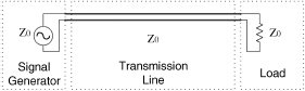
Figure 3.2 is a matched transmission line system. On the left side is a signal generator with a source impedance of Z₀. On the right side is a load whose impedance is also Z₀. A transmission line of parallel wires with characteristic impedance Z₀ connects the signal generator and the load. In a system like this, impedances at both interfaces, between the signal generator and the transmission line and between the transmission line to the load, are perfectly matched. The electromagnetic energy transfers from the generator to the load through a pure form of traveling wave. Whenever energy travels in a transmission line, it induces currents. Can we draw the conclusion that a transmission line radiates? The answer is no. A transmission line does not radiate in its designated working frequency band, which is from DC (direct current) to a certain frequency point. To explain that, we need to investigate the current distribution in a matched transmission line system.

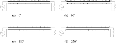
Figures 3.3a–d are transient current distributions at four different phase angles, 0°, 90°, 180°, and 270° respectively. The current distribution varies with a period of 360°. The length of the transmission lines shown in all four figures is one wavelength. The arrows in the figures represent the direction of currents. The length of each arrow represents the current's amplitude at corresponding location. Figure 3.3a shows the transient current distribution when the phase angle is 0°. It can be seen from Figure 3.3a, there are currents in both wires of the transmission line. The current in the same wire reverses its direction every half-wavelength. At any given location, the currents in both wires are always the same in amplitude and the opposite in direction.

In theory, each current can generate a radiating electromagnetic field in the whole space. However, if the working frequency is low enough, the two currents in opposite directions generate two radiating electromagnetic field with complete reversed polarities. Based on the superimposition principle, the actual electromagnetic field induced by a transmission line is zero everywhere. That means a transmission line cannot radiate at low frequency.

Figure 3.3b shows the transient current distribution when the phase angle is 90°. Compared to Figure 3.3a, it is clear that the electromagnetic wave is propagating along the transmission line in a purely traveling wave mode and the propagating direction is from left to right. In Figure 3.3b, currents in both wires are also the same in amplitude and the opposite in direction. So the transmission line still cannot radiate at low frequency. Similarly, currents in Figures 3.3c and d cannot radiate.

Based on Figures 3.3a–d, let's try an interesting exercise. Try to imagine an animated film; in the film, the current distribution starts as shown in Figure 3.3a, then the current continuously spreads to the right until it appears to be same as the current shown in Figure 3.3b. Keep the current moving to pass the status shown in Figure 3.3c. Figure 3.3d, and then Figure 3.3a again to finish a full cycle. This practice can help us better understand the process of energy propagation in a transmission line.

There is always a distance difference between any given location to these two wires. As is well known, the electromagnetic wave travels with a limited speed and the phase of an electromagnetic wave varies 360° every wavelength. When the frequency is so high that the signal's wavelength is comparable to the gap between two wires, the phase difference caused by the gap cannot be ignored, then that 180° relationship is also broken and the transmission line starts to radiate.

Next, let's look at a transmission line without a load. Using a water pipe as an analogy, similar to a water pipe which can constrain the water's flow without leaking, a transmission line can constrain energy's flowing without radiating. In our real life experience, one can let the water out by turn on the faucet. Is it possible to radiate electromagnetic energy from the transmission line by simply removing the load or terminator shown in Figure 3.2 ? The answer is still no. Unlike water which can flow through a faucet, electromagnetic wave spreading to the right is completely reflected back at the location of the open circuit. The reason for the reflection is due to the mismatch between the characteristic impedance Z₀ and the impedance of the open circuit, which is +∞. A detailed explanation is omitted here and can be found in references [1–4].

The incident wave propagating to the right and the reflected wave spreading to the left match in the transmission line to form a standing wave. Figure 3.4 shows the transient current distributions of a standing wave on an open circuit transmission line. Figure 3.4a–d are transient current distributions at four different phase angles. At the right end of the transmission line of all four figures is the open circuit, and the current is always 0. In the middle of the transmission line which is half a wavelength away from the open circuit there is another spot where the transient current is always 0. In fact, in all locations where the distance to the open circuit is an integral multiple of half a wavelength, the transient currents there are always 0. The terminology of all these points is the wave node. At all locations where the distance to the open circuit is an odd multiple of a quarter of wavelength, the absolute amplitude of current is always the maximum. These points are called the wave crest. Because a standing wave is formed by superposition of both an incident and a reflected wave, its maximum amplitude is twice as much as the maximum amplitude of the incident wave.

Now we can look at the transient current of a standing wave. In Figure 3.4a when the phase angle is 0°, the current at all places along the transmission line is 0. Then amplitudes of current at all places start to increase proportionally. However, the wave is not traveling and it always stays in the same place. The absolute amplitudes of current at all locations reach their extreme when the phase angle is 90°, which is shown in Figure 3.4b. The maximum current appears at all wave crests. The current is twice as much as the current shown in Figure 3.3 when the signal generator injects the same amount of power.

Similar to Figure 3.3, the current in the same wire reverses its direction every half a wavelength. At any given location, the currents in both wires are always the same in amplitude and the opposite in direction. It is obvious that those currents cannot generate a radiating field. After the phase angle passes 90°, amplitudes of current at all places start to decrease proportionally. They become 0 again when the phase angle is 180°, as shown in Figure 3.4c. They reach another extreme at 270°, as shown in Figure 3.4d. Comparing Figures 3.4b and d, it can be seen that although currents in both status reach their extreme, the directions of the current are all reversed.

So far, we have stated that a matching transmission line does not radiate and neither does an open circuit transmission line. It is easy to prove that a short circuit transmission line or a transmission line with any kind of loading could not radiate.

To design something to radiate, we have to find some structures which can carry currents, and far fields generated by these currents do not totally cancel each other. Figure 3.5 shows a dipole antenna fed by a parallel wire. Actually this structure can also be converted from an open circuit transmission line. By bending wires at the open end of the transmission line by 90° and keeping them apart, we get the structure shown in Figure 3.5. To decide the current on the dipole antenna, we need Kirchhoff's current law, which states that in an electric circuit the algebraic sum of all the currents flowing out of a junction is zero. Without loss generality, we can assume the current on the top wire is going toward the right. Based on Kirchhoff's current law, the current direction on the top arm of the dipole is up. Because the currents are always in the reverse direction on wire pairs of a transmission line, the current on the bottom wire is to the left. Then the current direction on the bottom arm of the dipole can also be decided and this is up.

It is now clear that the current directions at any given location on both arms of the dipole are all the same. Instead of canceling each other out, fields generated by currents enforce each other in the outer space. By bending the end of transmission line, we obtain an antenna. To be able to radiate effectively, a basic dipole antenna has to meet another requirement, which is that the total length, L, needs to be half a wavelength.

Figure 3.6 shows a simulation result of a dipole antenna. The antenna's length, L, is designed to be half a wavelength at f₀. In the simulation, a 50 Ω is used as the source impedance of signal generator. The simulated frequency range is from 0 to 8∗ f0. The Y axis in Figure 3.6 is the reflection coefficient, for which the lower the better. There are two X axes. The upper X axis is the relative frequency normalized by f₀, which is from 0 to 8. Because the frequency is inversely proportional to the wavelength, the X axis can also be represented by the wavelength. The lower X axis is the ratio between the antenna length L and wavelength λ.

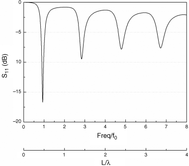
It can be seen from Figure 3.6a, dipole antenna cannot cover all frequency bands. It only periodically achieves good matching. Here, a reflection coefficient lower than −5 dB is considered good matching. Based on the theory with some simplifications, besides the base frequency f₀, a half-wavelength dipole also radiates well at 3∗ f₀, 5∗ f₀, and any odd multiple of the f₀. That can be verified by the simulated results shown in Figure 3.6. One might notice that the resonant frequencies of simulated result are around but not exactly at the odd multiple of f₀. That is the usual difference between theory and practice. In theory, everything is perfect. In reality, the end of the dipole antenna always has some distributed capacitance which effectively loads the antenna and makes the resonant frequency lower. However, in practice, it is not really an issue at all, we can just tune the antenna length to get the right frequency.

Figure 3.6 can also be described from the wavelength point of view. When the dipole length is half a wavelength, it is well matched. When the length of a dipole is 1.5λ, 2.5λ, and any odd multiple of half a wavelength, it can also effectively radiate. Shown in Figure 3.7 are current distributions of a dipole antenna at f₀ and 3∗ f₀. The rightmost graph is the color bar of current amplitude. At frequency f₀, there is only one standing wave. The current's amplitude is 0 at both ends of the antenna and it reaches the maximum in the middle, where the feed point is. At frequency 3∗f₀, there are three standing waves. The current's amplitude reaches the maximum at three locations. As shown in Figure 3.7b, the current on the antenna alternatively changes directions. Based on these two current distributions, it should be easy to work out distributions of other higher order modes.

The phenomenon of multiple resonances of a single antenna is very important and is widely used in designing multi-band antennas. We will leave this topic to later sections. For now, we'll focus on the lowest resonant frequency f₀.

Although a dipole used to be a widely adopted antenna form factor in the wireless communication industry, it is too cumbersome to be used in today's mobile phones. As a quantitative example, a dipole needs to be 182 mm long at 824 MHz, which is the band edge of the US cellular band. This length is much longer than any phone currently on the market, so we definitely need something shorter.

Using the dipole antenna shown in Figure 3.5 as the starting point, we can get the structure shown in Figure 3.8a by expanding the bottom arm of a dipole antenna. Then we can remove the transmission line and replace it with a signal source directly placed between the top “normal” arm and the bottom “fat” arm. The final transformed new antenna structure is shown in Figure 3.8b. It may still look like a dipole antenna, but the name of the antenna changes to monopole antenna now, because from the point of view of a system engineer or a project manager, the bottom arm does not belong to antennas. In a real phone, the bottom arm actually is a piece of the printed circuit board (PCB), where all the circuit components, such as all kinds of integrated circuits (IC), resistors, capacitors, and inductors are mounted. Except for a few matching components, an antenna engineer can change practically nothing on that board. The board's specific dimensions, such as length, width, and thickness, are all decided by engineers from other disciplines.

A PCB board normally has a multi-layer structure. It is composed of layers of insulating sheet and copper traces laminated by pressing processes. In the mobile phone industry, four-layer, six-layer, and eight-layer boards are widely used. The number of layers shows how many layers of copper traces it has. To eliminate noise and electromagnetic compatibility issues, normally there is a ground layer inside the PCB lamination. From the antenna's point of view, the ground layer is the dominant radiator and the whole board can be simplified as one piece of metal.

In a structure as shown in Figure 3.8b, only the top arm is considered an antenna, so the total length of a monopole antenna is a quarter of a wavelength instead of the half a wavelength required by a dipole antenna. But we must always remember that the PCB is the other half of an antenna. Without a PCB, any monopole antenna would not work. The size of a PCB should be larger than an antenna, otherwise the antenna might have problems at low frequency.

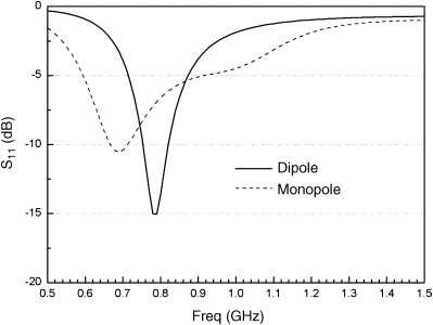
For the purpose of comparison, the simulated results of a dipole and a monopole antenna are shown in Figure 3.9. The total length of the half a wavelength dipole is 180 mm, and each arm is 90 mm. The resonant frequency of the dipole antenna is 790 MHz, which is lower than the 830 MHz predicted by the half a wavelength assumption. The length of the quarter of a wavelength monopole antenna is 90 mm. The PCB on which the whip monopole is installed is simulated by a perfect conductive sheet with the dimensions of 70 mm∗120 mm as shown in Figure 3.8b. Although both the dipole and the monopole have identical top arms, the resonant frequency of the monopole antenna is 690 MHz, which is lower than the dipole's. That is due to the effect of the PCB. Compared with a dipole antenna which has a 90 mm-long bottom arm, the PCB is 120 mm long and it makes the whole radiating structure bigger and drives the resonant frequency lower.

Although a whip monopole antenna is only half the size of a dipole antenna, it is still too big to be used as a fixed antenna on a mobile phone. Now it is the time for helix monopole antennas to enter the stage. As we know that the resonant frequency of a monopole antenna is roughly decided by the length of wire, it is quite natural to think about coiling the wire round to make a helix. Figure 3.10 shows a helix. The critical dimensions to define a helix include the pitch P, the diameter of the helix D, the diameter of the metal wire d, and the total number of turns N.

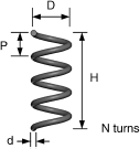
The total wire length of a helix can be expressed by Equation (3.2):

(3.2)

The total height of a helix H can be expressed by Equation (3.3):

(3.3)

By adjusting D, P, and N, any required length can be obtained. However, even with the same wire length, different helixes have different frequency response. Some parametrical studies will be presented in following figures to demonstrate the effect of different parameters.

Figure 3.11 shows three 90 mm-long helixes with the same helix diameter of 6 mm and wire diameter of 1 mm. It can be seen from Equation (3.2), if the diameter of the helix is fixed, only the pitch and number of turns can be adjusted. The helix (a) has 3.5 turns and a pitch of 15.5 mm. The helix (b) has 4 turns and a pitch of 12 mm. The helix (c) has 4.5 turns and a pitch of 7 mm. The total height of helixes (a), (b), and (c) is 61.3 mm, 48 mm, and 31.5 mm respectively. Figure 3.12 shows the drawing of the helix (c) with a PCB which is identical to the one shown in Figure 3.8 b. All three helixes are simulated with the same PCB.

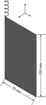
Figure 3.13 is the simulated results of a whip monopole and three helixes when installed on the same PCB. The result of whip monopole is the same as shown in Figure 3.9. Although all four antennas have the identical wire length, 90 mm, their resonant frequencies are different. With the decrease of an antenna's total height, the resonant frequency of the antenna shifts higher. However, the resonant frequency of a helix antenna is still much lower than a whip monopole with the same height. For example, the helix (c) resonates at 1.16 GHz and a 31.5 mm tall whip monopole resonates at 1.6 GHz.

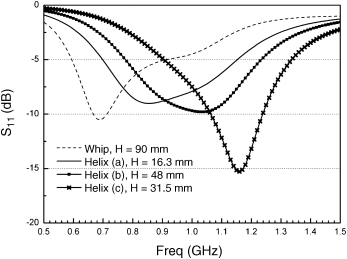
Figure 3.14 shows three 90 mm-long helixes with the same height of 31.5 mm and wire diameter of 1 mm. The diameters of helixes (a), (b), and (c) shown in Figure 3.14 are 9 mm, 7.5 mm, and 6 mm respectively. By fixing the height of a helix and the diameter of the helix, there is only one combination of pitch and number of turns which can produce the required total length. In Figure 3.14, the pitch of the helix (a) is 10.5 mm and the number of turns is 3. The pitch of the helix (b) is 8.8 mm and the number of turns is 3.58. The pitch of the helix (c) is 7 mm and number of turns is 4.5. The helixes (c) shown in both Figures 3.12 and 3.14 are identical.

Figure 3.15 is the simulated results of four antennas. The results of the whip antenna and helix (c) are identical to those shown in Figure 3.13. They are included for the convenience of comparison. Once again, four antennas with the same length have different resonant frequencies. When the height is fixed, an antenna with larger helix diameter has lower resonant frequency. However, the effect of helix diameter is much less than the effect of helix height. By increasing the helix diameter from 6 mm to 9 mm, the total volume of the helix is more than doubled. The frequency variation due to that amount of volume change is only 6.5%. When the helix height changes from 31.5 mm to 61.5 mm, the volume change is less than two times, but the frequency varies 36%.

So far, we have studied several different helixes under one constraint, which is that the total length of helix is always 90 mm. As a summary, whenever we try to coil a fixed length wire up to make a helix, the smaller the helix, the higher the resonant frequency. If the volumes of two same-length helixes are also the same, the resonant frequency of the taller and thinner one is always lower.

The ultimate goal when designing a helix antenna is to replace a whip monopole antenna, so a helix antenna must have the same resonant frequency as the one it needs to replace. To compensate for the frequency shift that any helix antenna inheres, the total wire length of a helix should be longer than the whip one it replaced. When the height and diameter of a helix are fixed, its resonant frequency can be tuned by adjusting the helix's turns. Based on Equation (3.3), its pitch also needs to be inversely proportionally adjusted.

As an example, a helix antenna with a height of 31.5 mm and a diameter of 6 mm is parametrically studied. By proportionally adjusting the number of turns and the pitch, different resonant frequencies can be obtained. Shown in Figure 3.16 is the simulated result of resonant frequencies vs. number of turns. By adjusting the helix's turns from 2 to 10, the resonant frequency changes from 1.45 GHz to 0.68 GHz. To replace a 90 mm whip monopole antenna, which is resonant at 0.69 GHz, a helix antenna needs roughly 10 turns when H = 31.5 mm and D = 6 mm.

Figure 3.17 shows the simulated result of resonant frequencies vs. wire's length of helixes. The simulated cases used in Figure 3.17 are identical to those used in Figure 3.16. However, the X axis in Figure 3.17 is replaced by the helix's length calculated by Equation (3.2). It is clear in Figure 3.17, to obtain the 0.69 GHz resonant frequency, the total wire length of the helix is 190 mm, which is more than twice the length of a 90 mm whip monopole.

In the real world, to design a whip monopole or a helix monopole antenna, one really does not need any parametrical study. To design a whip monopole, just cut a quarter-wavelength copper wire and solder it to the device. The resonant frequency should be lower than the theoretical one. That is what we want. We always start the tuning process of a monopole antenna at a lower frequency. Lower frequency means a longer radiator. It is much easier to cut copper wire off to shift the frequency up than to put wire back in.

When designing a helix antenna, the height and the diameter of the helix are normally already decided by industrial design (ID) engineers. For those not familiar with various disciplines of engineering, industrial design is a combination of applied art and applied science, whereby the aesthetics and usability of mass-produced products may be improved for marketability and production. They are the number one “enemy” who make antenna engineers suffer. They always want to remove any cosmetic trace of the existence of an antenna, and they are the ones who want to wrap the whole antenna with a shiny stainless steel cover. The “enemy” number two is mechanical engineers. They are responsible for creating the cosmetic design generated by industrial design engineers. Due to the consistent pressure from the marketing department to make mobile phones smaller and slimmer, mechanical engineers always find themselves in an embarrassing situation; it seems that there is never enough space to squeeze all the stuff in. Naturally, mechanical engineers will conspire to “steal” space allocated to antennas. To be an antenna engineer, part of the job's responsibility is to convince all the others that there is a undisputed reason for the reserved antenna volume and to communicate the minimum volume that must be retained in order to achieve the required antenna performance.

Similar to a whip antenna, to design a helix antenna, we can start with a half a wavelength wire, and then coil it to the wanted diameter and stretch it to the required height. This should generate a resonant frequency lower than what we want. The tuning process is cutting a little of the helix and stretching it to the correct height. Repeat the process until the correct frequency response is obtained.

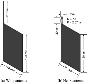
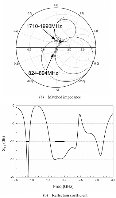
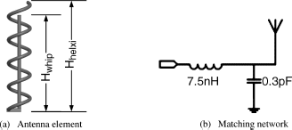
As a demonstration, we will design two single band antennas, a whip and a helix, for phones used in the US market. That means that both antennas need to have a working frequency band covering 824 MHz to 894 MHz. A reflection coefficient less than −10 dB is used here as the specification to calculate the bandwidth. Through the cutting and measuring processes, the dimensions of the whip and the helix can be decided. The final dimensions of both antennas are shown in Figure 3.18. Both antennas are made of 1 mm copper wire. The whip antenna is 70 mm tall. The dimensions of the helix antenna are: H = 20 mm; D = 6 mm; P = 2.67 mm and N = 7.5 turns. The total wire length of the helix is 142 mm.

Shown in Figure 3.19 are the reflection coefficient results of both the whip antenna and the helix antenna. The reflection coefficient of the whip clearly shows a double resonance. The explanation for this phenomenon can be found in Section 3.5. The gray line segment is the specification line, which is −10 dB from 824 MHz to 894 MHz. The return loss of the helix meets the specification. All return loss value of the whip antenna is above −10 dB, which means the original whip antenna cannot meet the specification even at a single frequency point.

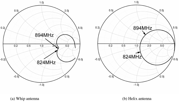
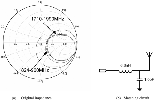
Does Figure 3.19 give us enough information to make the judgment on whether the helix antenna has a better performance than the whip antenna? Not really. When we talk about an antenna's performance, we actually refer to both its efficiency and its bandwidth. To evaluate an antenna's efficiency, an anechoic chamber must be used. To predict an antenna's bandwidth, the locus of impedance shown in a Smith Chart is required. Shown in Figure 3.20 are the locus of impedance of both antennas. Two band edges, 824 MHz and 894 MHz, are marked in both Figures 3.20a and b. It is clear that the bandwidth of both antennas can be improved by adding matching circuits.

Among the many factors which decide an antenna's achievable bandwidth, the following two are the most important and have the most influence:

• The length of impedance locus between two band edges. The shorter the length is, the easier it is to achieve wide bandwidth. What a normal matching circuit does is move the locus of impedance around on the Smith Chart. If an antenna has long impedance's locus, whenever one of the band edges is matched, the other band edge moves out of the center of the Smith Chart. Of course, the bandwidth expanding techniques introduced in Chapter 2 can be used to bend an impedance locus, thus achieving a wider bandwidth. As shown in Figure 3.20a, the locus length of the whip antenna between 824 MHz and 894 MHz is quite short, so it is quite easy to significantly improve the whip's bandwidth by a matching network. On the contrary, the locus length of a helix antenna is relatively long, thus only limited improvement can be achieved through matching.
• The distance from impedance locus to the center of the Smith Chart. This distance actually is the amplitude of reflection coefficient Γ introduced in Chapter 2. The center of the Smith Chart corresponds to |Γ| = 0. The outermost boundary of the Smith Chart corresponds to |Γ| = 1, which means total reflection. It is obvious that the lower Γ is, the easier it is to achieve wide bandwidth. To move the impedance further on a Smith Chart, the frequency response of the matching circuit is steeper; as a consequence, the antenna bandwidth is narrower. It must be remembered that the distance to the center is not linearly related to the achievable bandwidth. Any impedance on the circle of |Γ| = 0.5, which has a reflection coefficient of −6 dB, is still pretty easy to match. As a comparison, the achievable bandwidth of an impedance on the circle of |Γ| = 0.9 is extremely narrow.

Combining the impact of both factors, it is safe to say that the whip antenna has a much wider bandwidth than the helix antenna.

Two circuits shown in Figure 3.21 are used to match the whip antenna and the helix antenna respectively. Both of them are simple two-element matching. For fairness of comparison, both circuits use the same topology.

Shown in Figure 3.22 are the reflection coefficient results of the matched whip and the matched helix. With a matching circuit, the −10 dB bandwidth of the helix antenna increases from 80 MHz to 110 MHz. Meanwhile, the bandwidth of the matched whip increases to 560 MHz, and it covers 0.74 GHz–1.3 GHz.

It is now clear that it is not a free lunch to compress an antenna into a smaller volume. With the decrease of the antenna's volume, the bandwidth shrinks rapidly. For a helix antenna, decreasing the diameter D or the height H shrinks its bandwidth. However, decreasing a helix's height has more impact on its bandwidth.

Some might have noticed that there are dual resonances in the whip's frequency response. This is due to both its unsymmetrical structure and its wideband characteristic. The whip and the PCB are two equivalent arms of a dipole antenna. They are different in dimension, so each of them has their own resonant frequency. When both resonances have a wideband characteristic, their combined frequency response has dual resonances. That happens to be the case in a whip antenna. In comparison, a helix antenna is also asymmetric, but the bandwidth of a helix is so narrow that its frequency response conceals the resonance of a PCB. This is the reason why a small helix antenna always has a clean impedance locus.

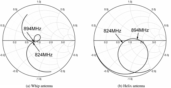
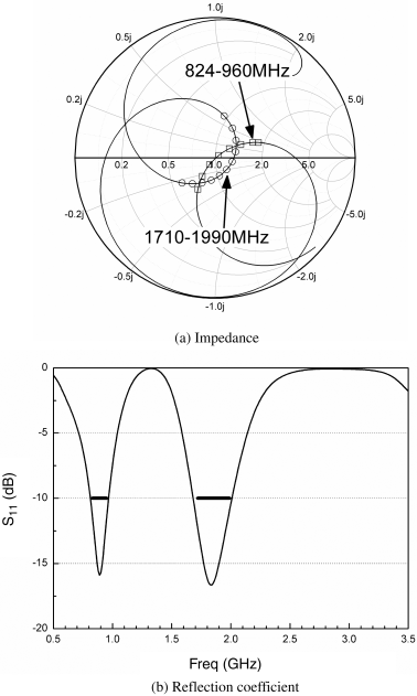
Shown in Figure 3.23 are the impedance's loci of the matched whip and the matched helix. It can be seen that the loci between 824 MHz and 894 MHz of both antennas are well positioned in the center of the Smith Chart. As a comparison, the original impedance in Figure 3.20b passes by the center from the right side of the Smith Chart. The locus of the matched helix moves around the center of the Smith Chart. That brings the whole locus closer to the center and thus provides wider bandwidth. Due to the wide frequency scale, it may not seem clear in Figure 3.22, a matching network still improves the helix antenna's bandwidth by about 30%.

Figures 3.24a–c are 3D radiation patterns of an ideal half-wavelength dipole antenna, a whip antenna and a helix antenna respectively. The axis of the dipole antenna is aligned to the Z-axis. The 3D pattern of the dipole looks like a donut. As shown in Figure 3.24a, due to its axial symmetrical property, a dipole's pattern is also axial symmetrical and has its peak located in the XY-plane. In Figures 3.24b and c, the axis of the whip and the helix are also aligned to the Z-axis. The PCBs of both the whip and the helix are placed in the YZ-plane. Both Figures 3.24b and c have the same angle of view as Figure 3.24a. It is clear that radiation patterns of both still have a null around Z-axis, but patterns are no longer symmetrical and are slightly tilted to different directions.

For the simplicity of studies, most antennas simulated in the book do not include plastic covers or supports. In practice, these features are necessary to ensure the antennas' mechanical robustness. The dielectric constant or permittivity of commonly used plastics is around 2.6∼4.5. Due to the loading effect of plastics, the resonant frequency of an antenna decreases. This frequency shift can easily be compensated for by making the antenna radiator shorter. The more important issue related to plastic is loss. Different plastics have different loss properties, which has the potential to degrade the antennas' efficiency significantly. If the difference in efficiency of an antenna with plastic and without plastic is more than 1 dB, we need to investigate the plastic. Of course, the antenna in both cases needs to be well tuned.

Shown in Figure 3.25 are the simulation results of a helix antenna with and without a plastic cover. The permittivity of the plastic is 3.2. The diameter of the plastic part is 9 mm and the height is 23 mm. For the purposes of comparison, the result of the antenna shown in Figure 3.18b is also included. In Figure 3.25b, the solid line is the result of the original helix and the dashed line is the response after the helix is insert-molded by plastic. Due to the loading effect, the resonant frequency shifted from 850 MHz to 730 MHz.

The following guidelines are given as the summary of helix antennas' design:

• Whip or helix antennas must be installed on a PCB to work properly.
• The height of a helix antenna is the most important parameter, which decides the antenna's performance. Taller is better.
• The diameter of a helix antenna also influences its performance. Larger is better. However, the diameter of the helix's wire has limited impact on its performance. Larger diameter can slightly improve the bandwidth.
• When a plastic support or cover is used, the antenna's resonant frequency shifts lower, and it must be compensated for.

3.1.2 Multi-Band Helix Stubby Antenna

When the penetration rate of mobile phones started to take off in the early 1990s, it seemed that the allocated frequency bands, 824–894 MHz in the United States and 880–960 MHz in Europe, would soon run out of channels. Countries around the world began allocating new frequency bands to accommodate the rapidly increased demand. Around 1995, Europe allocated 1710–1880 MHz and the United States allocated 1850–1990 MHz as the new personal mobile communication bands respectively.

As a consequence, single-band antennas finally reached the end of their life span. Any antenna needs to support at least two frequency bands. In the United States, that means 824–894 MHz and 1850–1990 MHz. In Europe, that means 880–960 MHz and 1710–1880 MHz. A world phone, also called a tri-band or quad-band phone, needs to support bands in both continents.

3.1.2.1 Multi-Branch Multi-Band Stubby Antenna

It has been demonstrated that a whip or a helix can function as an antenna. By putting two such radiating elements together, what we get is a multi-band antenna.

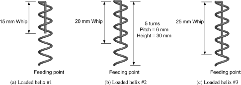
Figure 3.26 shows a two-branch stubby antenna. As shown in Figure 3.26b, the antenna is composed of an outer helix and an inner straight wire. Two radiating elements are connected together at the bottom. The heights of the whip and the helix are identical, both are 30 mm long. The helix's diameter is 6 mm; its pitch is 6 mm and it has 5 turns. Both elements are made of 1 mm-diameter copper wire.

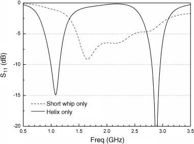
Shown in Figure 3.27 is the simulated reflection coefficient of the antenna. Around 0.9 GHz MHz, it has a clean sharp resonance, which is marked as (1). From 1.7 GHz to 2.9 GHz, the antenna has a wide response with several resonances, which is marked as (2). At 2.49 GHz, there is another sharp resonance, which is marked as (3).

Shown in Figure 3.28 are radiation patterns of the two-branch stubby antennas. At the low band, which is 0.88 GHz in this case, the radiation pattern is similar to a dipole's. The radiation is mostly generated by the vertical current along the ground plane. The vertical polarized electrical field E_θ is the dominant field component. At the higher band, which is 1.80 GHz, the E_θ and E_ϕ have the same order of amplitude. The field of E_θ is mostly generated by the current along the longer edge of the ground plane and the current on the antenna element. The field of E_ϕ is mostly generated by the current along the top horizontal edge of the ground plane, which explains why the radiation pattern of E_ϕ has a null along ±Y directions. Shown in Figure 3.28e is the radiation pattern of the total E field at 1.80 GHz. At the high band, the ground plane is relatively large compared with a quarter of a wavelength, thus some portion of current flows down along the vertical edge of the ground in a traveling wave's form factor, which in turn generates a downward-tilt radiation pattern. For cellular phones, it is quite safe to assume that at high frequency bands the peak of radiation pattern always tilts downward, away from where an antenna is installed.

The frequency response of a two-branch stubby has the contributions of both radiating elements. To distinguish the effects of two individual radiators and their mutual impact, the helix and the whip are separately simulated. Shown in Figure 3.29 are simulation results of a whip-only antenna and a helix-only antenna. Both antennas have identical specific dimensions like the antenna shown in Figure 3.26. In the figure, the helix-only antenna has two resonances, which are at 1.1 GHz and 2.9 GHz respectively. These two resonances correspond to modes of f₀ and 3∗ f₀. The whip-only antenna has a resonance between 1.5∼2.8 GHz. Comparing Figures 3.27 and 3.29, we can tell that resonances (1) and (3) in Figure 3.27 are generated by the helix and the resonance (2) is the contribution of the whip. When we put the two elements together, the helix is loaded by the whip, so resonant frequencies of both resonances (1) and (3) are 10% lower than its standalone version. The helix's bandwidth in both bands is also narrowed.

Now let's study a little bit more about the resonance (3) shown in Figure 3.27. From the return loss point of view, the helix resonance at 2.49 GHz, where the resonance (3) is found, has the best matching in the 1.7–2.9 GHz band. One might assume that the antenna also has the best efficiency at this frequency point. Unfortunately, this assumption is not correct. At 2.49 GHz, the antenna has the worst efficiency in the band.

Shown in Figure 3.30 is the radiation efficiency of the dual-branch antenna around 2.49 GHz. The simulated frequencies are zoomed in on the 2.0∼2.7 GHz range. The radiation efficiency is defined as the ratio between radiated power and accepted power by the antenna. Thus the radiation efficiency does not count in the mismatch loss. To simulate the loss effect, a block of lossy material (20 mm∗20 mm∗35 mm) is used to enclose the antenna. The permittivity of the material is 1 and its loss tangent is 0.01. The worst efficiency occurs at 2.49 GHz. Between 2.45 GHz and 2.55 GHz, the radiation efficiency is less than 80% and the reflection coefficient shown in Figure 3.27 is better than −10 dB. When the frequency is far from the 2.49 GHz, although the return loss value is around −7 dB, the radiation efficiency is better than 95%.

The reason for the low efficiency is not due to the helix element itself. The antenna efficiency is around 95% at 0.9 GHz, which is the first resonant frequency of the helix. The efficiency drop is due to the mutual impact between whip and helix. As shown in Figure 3.29, the whip itself has a quite wide resonance between 1.5 GHz to 2.8 GHz. Outside the close range of 2.49 GHz, the resonance of the two-branch antenna is mostly contributed by the whip. At 2.49 GHz, both the whip and the helix can resonate, that induces a self-resonance between themselves. In a whip and helix structure, the helix has a narrower bandwidth and it is outside the wideband whip, that makes its self-resonance stronger. When self-resonance happens, substantial amounts of energy are stored in the approximate area around the antenna. If an antenna is made of lossy material, which is always the case, this kind of self-resonance dissipates the signal energy on the lossy material.

When designing an antenna, we need to avoid the self-resonance frequency. It will be shown in the next section that the second resonance of a helix does not have to be 3∗f₀ and we have the means to move the helix's higher order resonance out of the working bands.

Now, let's finalize the design of the dual-branch antenna to provide tri-band coverage. The antenna needs to cover 824–894 MHz, 1710–1880 MHz, and 1850–1990 MHz. Shown in Figure 3.31a is the original impedance locus. The locus marked by hollow rectangular markers is the low band segment and the one marked by hollow circular markers is the high band segment. The filled circle is 2490 MHz, which has the best matching and worst efficiency. The matching circuit for this antenna is shown in Figure 3.31b. The original antenna already has a decent reflection coefficient at the low band, so the matching circuit is mostly for the high band.

Shown in Figure 3.32a is the impedance of the matched antenna. It is clear that the matching circuit moved both the high and low band. However, it moves the high band further. When designing an antenna, we always want to use the simplest matching circuit. That requires an integrated design procedure including both matching circuits and radiating elements. A matching circuit might shift an antenna's resonant frequency, so it is not necessary to fine tune the original antenna's frequency before a matching circuit is designed. After making the antenna roughly resonate at the right frequency, we can start to design the matching circuit. Then it is time to tune the antenna again. It normally takes a few iterations to get a satisfying design.

The results shown in Figure 3.32a are the result after a few iterations of tuning procedures. The 824–894 MHz band is well positioned near the origin of the Smith Chart. The best matched frequency in the lower band is 860 MHz. As a comparison, the best matched frequency in the lower band of the original antenna, as shown in Figure 3.31a, is 900 MHz and its low band locus is offset toward the lower half of the Smith Chart.

Figure 3.32b is the simulated reflection coefficient result. The two thick lines mark the −10 dB of 824–894 MHz and 1710–1990 MHz bands. The antenna barely meets the −10 dB specification at the low band and has large margin at the high band.

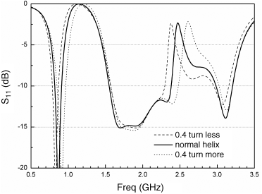
To tune the lower resonant frequency, we can adjust the total length of the helix. By decreasing the total turns of the helix and increasing the pitch accordingly, we can decrease the total length of the helix while keeping its height. Shown in Figure 3.33 is a parametric study of the impact of helix length. All three antennas have the same height and use the same matching network. The solid line represents the normal antenna. The dashed line and dotted line represent antennas with helixes 0.4 turns shorter and 0.4 turns longer respectively. It is clear that the helix's length mostly affects the lower band and it does not have too much impact on the 1.6–2.2 GHz band.

One might already have figured out that by adjusting the length of the whip, the higher band can also be tuned. In fact, the effect of the whip is a little bit more complex. As already shown in Figures 3.27 and 3.29, the whip also has a loading effect on the helix. When adjusting the whip, the lower band also shifts, so iterative tuning procedures of both bands have to be performed.

In the following example, we will design a quad-band antenna to cover 824–894 MHz, 880–960 MHz, 1710–1880 MHz, and 1850–1990 MHz bands. The antenna has the same outside dimensions as the tri-band antenna shown in Figure 3.26b. By simply looking at the reflection coefficient of the tri-band antenna shown in Figure 3.32b, we can tell it is not difficult to design a quad-band antenna. To understand why, we must first understand one of the most important trade-offs in antenna design, which is the trade-off between different bands.

To master the art of designing any type of multi-band antennas, we must at least learn two techniques. The first is how to generate multiple resonances and how to tune their frequency separately, which we have already discussed. The second is how to trade off the bandwidth between different bands.

Sometimes one might find an antenna does not meet the specifications in one band and has a huge margin in the other band. This most likely means the antenna's design engineer does not understand the bandwidth trade-off of that kind of antennas. For most antennas, such a trade-off is always possible.

For a dual-branch antenna, the critical parameter when exchanging bandwidth is the height ratio between helix and whip. The height ratio between a whip and a helix is in direct proportion to their bandwidth ratio, as shown in Equation (3.4):

(3.4)

Shown in Figure 3.34a is the optimized quad-band antenna. The height of the antenna, which is now decided by the height of the helix, is still 30 mm. The length of the whip has decreased to 26 mm. After iteratively adjusting the helix and the matching circuit, a quad-band coverage is achieved. The final helix has 4.6 turns and its pitch is 6.52 mm. The matching network is shown in Figure 3.34b.

Shown in Figure 3.35 is the reflection coefficient of the quad-band antenna. The reflection coefficient of the tri-band antenna is also included for comparison. By decreasing the whip's length, the −10 dB bandwidth of the lower band increases from 70 MHz to 136 MHz. In the meantime, the −10 dB bandwidth of the high band decreases from 830 MHz to 470 MHz.

In fact, the quad-band antenna we have just designed still does not fully exploit the potential of the antenna's volume. There are different ways to expand the working bandwidth of both bands simultaneously. Shown in Figure 3.36a is one such example, it is an antenna with a metal base. The metal base is 10 mm long. The height of the helix is 20 mm long. This antenna has the same outer dimension as both antennas discussed above. Shown in Figure 3.36b is the antenna's matching network. Compared with the quad-band antenna, the antenna with a metal base has an even wider bandwidth at both low and high bands.

The following guidelines are given as the summary of multi-branch helix antennas' design:

• The higher and lower resonances of a dual-branch antenna are relatively independent. The whip decides the frequency of higher resonance and the helix decides the lower one.
• The bandwidth between higher and lower band can be exchanged by adjusting the relative height between the whip and helix. Increasing the height of one can expand its corresponding bandwidth
• The metal base can be used to expand the bandwidth of both bands.

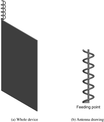
Shown in Figure 3.37 is a dual coil helix antenna. It is also a multi-branch antenna. The center wire is replaced by a coil. As shown in the mechanical drawing, two coils and the metal contact are effective radiators. All plastic parts are used for the purpose of mechanical durability. By looking at the design, it is easy to tell that more consideration was given to the low band.

3.1.2.2 Single-Branch Multi-Band Stubby Antennas

In this section we are going to introduce multi-band stubby antennas composed of only one piece of wire. To generate multiple resonances on a single radiator, the higher order mode of that radiator must be used. The concept of a dipole antenna's higher order modes has been detailed in Figure 3.6. The conclusion is that if the resonant frequency of a half wavelength dipole antenna is f₀, the dipole can also be resonant at 3∗f₀, 5∗f₀ and all other odd multiples of f₀.

The higher order mode resonances are not an exclusive property of dipole antennas. A helical antenna also has the similar characteristic. In fact, higher order modes are nothing unique and they exist in all kinds of antennas.

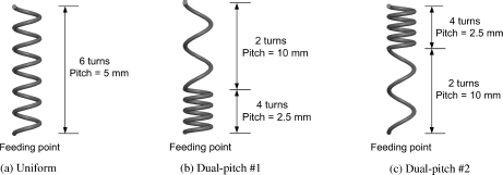
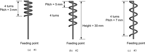
Let's start from dual-pitch antennas. As it is a widely used antenna configuration, several companies hold related patents [5–7]. Shown in Figure 3.38 are three variants of six-turn helixes. All of them have same diameter (6 mm), total height (30 mm), and number of turns. They are all fed from the bottom. Shown in Figure 3.38a is a uniform pitch helix. Shown in Figure 3.38b and Figure 3.38c are two dual pitch helixes. The dual-pitch #1 helix has two turns of large pitch (10 mm) and 4 turns of small pitch (2.5 mm). The height of the large pitch and the small pitch segments are 20 mm and 10 mm respectively. The #2 helix is similar to the #1 except its large pitch segment is at the bottom.

Shown in Figure 3.39 are results of above three helixes. Let's use the uniform helix as the base line. The first resonance of the uniform helix is at 0.95 GHz and the second one is at 2.5 GHz. That means the second resonance is at 2.6∗f₀, instead of 3∗f₀. This is due to the asymmetric characteristic of the structure, which is composed of both a helix and a PCB. By compressing the bottom portion of a uniform helix and stretching its top portion, we have the #1 antenna. Compared with the uniform helix, the #1 antenna resonates at a lower frequency at the low band and at a higher frequency at the higher band. On the contrary, the #2 antenna has a reverse relationship to the uniform helix. It has a higher resonant frequency at the low band and a lower resonant frequency at the higher band.

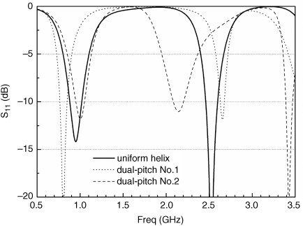
Listed in Table 3.1 are the ratios between the second and the first resonant frequencies of all three antennas. It is clear that we can separate the first and the second resonant frequencies by squeezing the bottom portion of a helix. If we squeeze the top portion of a helix, we can make two resonant frequencies closer.

Table 3.1 Frequency ratio of different dual pitch antennas

Antenna type	Ratio between second and first resonant frequency
Uniform	2.6
Dual-pitch #1	3.3
Dual-pitch #2	2.1

In Figure 3.30, we discussed the efficiency drop of a whip–helix antenna due to the helix's second resonance. It is obvious that by using a dual-pitch helix, the second resonance can be moved around to avoid any negative impact inside the working band.

In the North American market, a dual-band antenna needs to cover 824–894 MHz and 1850–1990 MHz, which has a relative ratio of 2.2. In the European market, an antenna covers 880–960 MHz and 1710–1880 MHz, the relative ratio is 2.0. Both standards require a ratio less than 2.6, which is the ratio of a uniform pitch helix. So for mobile phone antennas, what we need are dual-pitch helixes with a squeezed top portion.

There are many parameters which can be adjusted in the design of dual-pitch antenna. The effect of some parameters is the same for both uniform and dual-pitch helixes. Such parameters include the helix's height, the total wire's length, the number of turns, and the helix's diameter. All of them have been investigated elsewhere and are not discussed here.

Now let's focus on the two most important issues of antenna designing: (1) How to tune frequencies?; (2) How to exchange bandwidth? Let's start with the first one. As we already know, by adjusting the total length of a helix's wire, the lowest frequency can be changed. To be able to tune both the low and high bands simultaneously, what we need is a way to adjust the ratio between the first and the second resonance. This can be achieved by changing the pitch ratio between two segments.

To illustrate the effect of pitch ratio, three antennas as shown in Figure 3.40 are simulated. All three helixes have the dimensions except the pitch ratio. They have two turns of large pitch helixes and four turns of small pitch helixes; the total height is 30 mm. There are slight differences in wire length (≈117 mm), which can be calculated by Equation (3.2), among three helixes. The effect of this length difference can be ignored.

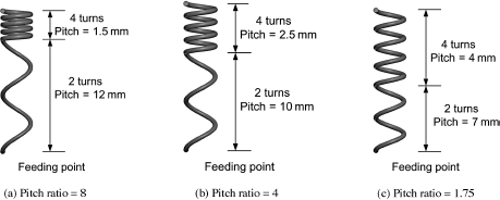
The antenna shown in Figure 3.40b is the same one shown in Figure 3.38c, and it is used as the normal sample. The pitch ratio between the large and small pitches are 8, 4, and 1.75 for three antennas respectively.

Results of three helixes are shown in Figure 3.41. By adjusting the pitch ratio, we are able to change the ratio between the first and the second resonance. The frequency ratios between the second and the first resonances of three helixes are 1.7, 2.1 and 2.5 respectively. When the pitch ratio changes, the frequency of the first resonance is relatively stable and the second resonance drifts in a wide range.

Now let's discuss how to exchange bandwidth between bands. The critical parameter here is the ratio of number of turns between large-pitch and small-pitch portions. All three helixes have the same height, diameter and number of turns. The antenna shown in Figure 3.42b is the same one shown in Figure 3.38c, and it is again used as the normal sample. In this comparison, the heights of both small-pitch and large-pitch portions are kept unchanged, which are 10 mm and 20 mm respectively. What is changed is how many turns of the helix are put in each portion. In the top portion, three antennas have 3, 4, and 5 turns of helix respectively. One might have noticed that when the turn-ratio changes the pitch-ratio also changes. As a result, when the bandwidth is exchanged between low and high bands, their frequency ratio is also altered. It is obvious that an iterative procedure must be included to compensate for this effect.

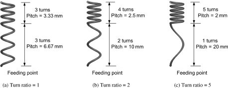
As shown in Figure 3.43, by decreasing the number of turns at the large-pitch segment, we are able to decrease the bandwidth at the lower band in exchange for wider bandwidth at higher band. The antenna shown in Figure 3.42a has the widest low band and the narrowest high band. On the contrary, the antenna shown in Figure 3.42c has the narrowest low band and the widest high band. As the median sample, the Figure 3.42b antenna's bandwidth at both bands is moderate among all three.

Now let's use the helix shown in Figure 3.40a as the radiator element to finalize a quad-band antenna design. The antenna also needs to cover the 824–894 MHz, 880–960 MHz, 1710–1880 MHz, and 1850–1990 MHz bands. Shown in Figure 3.44 is the original impedance locus of the Figure 3.40a antenna. The locus marked by hollow rectangular markers is the low band segment and the one marked by hollow circular markers is the high band segment. Compared with a dual-branch antenna, as shown in Figure 3.31a, the impedance locus of a single-branch helix is more regular. At a very low frequency, the antenna is too small to have any effect, so the antenna likes an open circuit and its impedance is close to infinity. At each resonant frequency, the antenna's impedance moves through a circle. There are three circles in Figure 3.44, they correspond to resonance at 0.95 GHz, 1.7 GHz, and 3.1 GHz respectively, as shown in Figure 3.41.

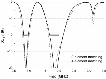
Shown in Figure 3.45a is a 3-element matching circuit and Figure 3.46a is the matched impedance with this circuit. Shown in Figure 3.45b is a 4-element matching circuit and Figure 3.46b is the matched impedance with this circuit.

Shown in Figure 3.47 are results of the matched Figure 3.40a antenna. Both matching circuits can meet the −10 dB quad-band specification. The bandwidth of the low band of a 3-element matching marginally meets the specification, which can also be observed from Figure 3.46a, as both bands are not centered in the Smith Chart. By increasing one more matching component, the antenna's matching is improved. In reality, to decide which matching is better, some chamber efficiency measurements are necessary. Because the extra component also introduces extra losses, only chamber measurements can evaluate these two counteracting effects.

So far we have discussed dual-pitch helixes. Of course, you can make a multi-pitch helix, which introduces more design variables and makes the design procedure more complex. In my opinion, it is not necessary to use multi-pitch helixes in a dual band design. Only when you need to cover multiple separated frequencies, say, 1 GHz, 2 GHz, and 5 GHz, can multi-pitch helixes be considered. You can also use a whip-helix antenna introduced in Section 3.1.2.1. By replacing the uniform helix with a dual-pitch helix, the lowest and highest band can be covered. By adjusting the whip's length, the middle band can also be covered.

The following guidelines are given as the summary of dual-pitch antenna's design:

• Although the parametrical studies are omitted on the effect of the height and diameter of dual-pitch antennas, they are all critical parameters which affect bandwidth. Increasing a helix's height can significantly expand its bandwidth; the only issue here is nobody likes a big antenna. Increasing diameter can moderately increase bandwidth.
• The frequency of the first resonance is mostly decided by the total length of the wire. The second resonance can be adjusted by changing the pitch ratio between small-pitch and large-pitch segments.
• To exchange the bandwidth between low and high bands, the ratio between the number of turns at small-pitch and large-pitch segments needs to be changed.
• Similar to the structure shown in Figure 3.36a, a metal base can increase an antenna's bandwidth.

Besides the dual-pitch helix, there are other ways to achieve dual resonance. The helix-loaded whip antenna, as shown in Figure 3.48, is one such example. For a traditional helix load whip, the helix is located on the end of a whip and extends upwards. The total height of such an antenna equals the sum of the heights of helix and whip. The helix load whip introduced here is different, and the helix goes downwards. That makes the antenna smaller; the antenna's height equals the height of the whip.

For this antenna, we will focus on the frequency tuning technique. To exchange bandwidth between bands, the distance between whip and helix needs to be changed. If the diameter of the helix is fixed, the whip must be biased from the axial line of the helix. An asymmetrical part like that is not easy to manufacture, so we will not discuss how to design it.

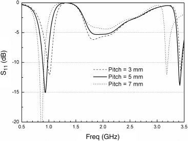
Shown in Figure 3.48 are three helix load whips. All of them have the same height (30 mm), the helix's diameter is 6 mm and number of turns is 4. They are all made of 1 mm diameter copper wire. The difference between them is the pitch of helix, which is 3 mm, 5 mm, and 7 mm for the #1, #2, and #3 antennas respectively. The total wire lengths of three antennas are almost same, which are 109 mm, 111 mm, and 113 mm respectively.

Shown in Figure 3.49 are the reflection coefficient results of the three antennas. By stretching the pitch of the helix from 3 mm to 7 mm, the antenna's low band resonant frequency shifts from 1.02 GHz to 0.87 GHz. In the meantime, the high band resonance maintains a relative stable location. The overall effect of changing the helix pitch is to adjust the frequency ratio between low and high bands. The other tuning parameter is the total wire length. By decreasing or increasing the wire length, the high and low bands can be simultaneously shifted higher or lower. Combining both parameters, we are able to allocate low and high bands to any required frequencies.

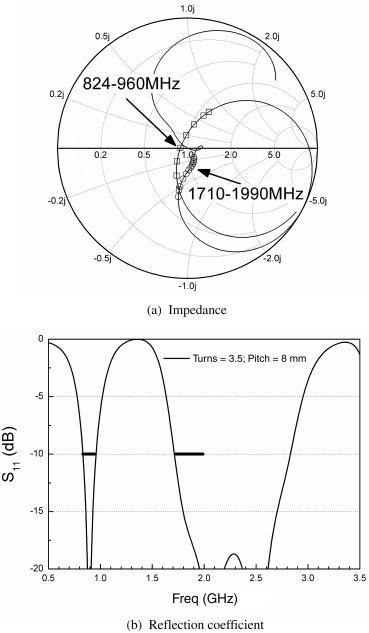
Now let's use the helix load whip structure to design a quad-band antenna. The antenna also needs to cover 824–894 MHz, 880–960 MHz, 1710–1880 MHz, and 1850–1990 MHz bands. The antenna used here is 30 mm tall. It has a 3.5 turn and its pitch is 8 mm. Shown in Figure 3.50a is the original impedance locus. The locus marked by hollow rectangular markers is the low band segment and the one marked by hollow circular markers is the high band segment. Shown in Figure 3.50b is a two-element matching network. The network is mostly for the high band's matching. However, it still shifts the resonant frequency at a low band even lower. To compensate for the shift, the original antenna is tuned to resonate at 940 MHz.

Shown in Figure 3.51a is the impedance of the matched antenna. Figure 3.51b is the reflection coefficient of the matched antenna. The antenna's reflection coefficient is −9.5 dB at the band edge of the low band and it does not meet the −10 dB specification. However, it has a huge margin at high band. The −10 dB bandwidth of the high band is more than 1 GHz, it covers from 1.71 GHz to 2.83 GHz.

The high band's reflection coefficient of an unmatched helix-loaded whip antenna is only around −5 dB, as shown in Figure 3.49. If we only look at the return loss result, it is very easy to get a false impression that this structure has limited bandwidth at high band. The wide band property at the high band can be easily observed on the Smith Chart, because the locus is concentrated in a very small area. This example reminds us whenever we design an antenna; we need to use two legs, both reflection coefficient results and impedance locus on the Smith Chart should be utilized.

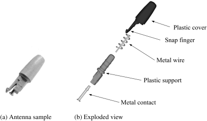
Shown in Figure 3.52 is a production single-branch stubby antenna. The coil and the metal contact are effective radiators. All the plastic parts are used for mechanical purposes. The snap finger is a feature to mechanically mate an antenna to a phone. In this design, the snap finger is integrated with the plastic cover and molded onto the antenna in one shoot.

Now let's check out one more way to design a dual-band antenna. Shown in Figure 3.53 are three whip load helixes. The antenna is changed from a uniform-pitch helix by attaching a straight vertical segment to the end of helix. All three elements have the same dimensions apart from the whip length. They are 30 mm tall. The diameter of helixes is 6 mm. The pitch is 6 mm and the number of turns is 5. The whip length is 15 mm, 20 mm, and 25 mm for the loaded helix #1, #2, and #3 antenna respectively. The total wire length is 117 mm, 122 mm, and 127 mm respectively. For the same reason as the helix load whip antennas, only frequency tuning techniques are discussed here and the means of exchanging bandwidth are omitted.

Shown in Figure 3.54 are the reflect coefficient results of the three antennas. By increasing the whip's length, the resonant frequencies of both low and high band become lower. Between the two bands, a whip has more impact on the high band. When the whip grows 10 mm (from 15 mm to 25 mm) the resonant frequency at the high band shifts 430 MHz (from 2.10 GHz to 1.67 GHz). And the ratio between the two bands changes from 2.0 to 1.83. The other tuning parameter is the total wire length. By decreasing or increasing the wire length, the high and low band can be simultaneously shifted higher or lower. Combining both parameters, we are able to allocate low and high bands to any required frequencies.

As a comparison, the whip-loaded helix in Figure 3.53c is used to design a quad-band antenna. Shown in Figure 3.55a is the original impedance locus. Shown in Figure 3.55b is a two-element matching network.

Shown in Figure 3.56a is the matched antenna's impedance. The Figure 3.56b is the reflection coefficient of the matched antenna. The antenna meets the −10 dB reflection coefficient specification of both bands with some margin.

So far, three single-branch multi-band antennas, the dual-pitch helix, the helix-loaded whip, and the whip-loaded helix have been introduced. A rational question one may ask is which we should select. For the convenience of comparison, the results from Figures 3.47, 3.51 and 3.56 are combined into Figure 3.57. It is clear that the bandwidth of the helix-loaded whip is the narrowest at the low band and the widest at the high band. On the contrary, the whip-loaded helix has the widest and narrowest bandwidth at the low and high bands respectively. The bandwidths' difference of three antennas at low band is limited, but their difference at high band is significant.

The bandwidth of a dual-pitch antenna can be adjusted by many parameters, so it is quite easy to design an antenna with well-balanced low and high bands. The potential issue with this kind of antenna is in the production. The antenna is sensitive to the pitch variation, especially at the small pitch segment. For example, if an antenna has a pitch of 1.5 mm and its wire diameter is 1 mm, then the smallest gap between the wires is only 0.5 mm. A 0.1 mm variation means 20% change on the gap. When designing a dual-pitch antenna, remember to give it enough margin on bandwidth.

The helix-loaded whip has an impressive wide high band. With enough height, it is easy to design an antenna whose high band is able to cover 1.575 GHz–2.5 GHz, which includes GPS (1575 MHz), DCS(1710–1880 MHz), PCS(1850–1990 MHz), UMTS(1920–2170 MHz), and Wireless LAN/Bluetooth(2400–2484 MHz). The shape of a helix-loaded whip may look difficult to make, in fact it only costs a few pennies (US$) if an experienced vendor can be found. The disadvantage of this antenna is its narrow bandwidth at low bands. If the bandwidth at low bands is critical, choose one of the others.

The whip-loaded helix has the narrowest high band. That is not always a disadvantage. Due to concerns about electromagnetic compatibility, sometimes a limited bandwidth is a good thing. A wideband antenna can pick up many out-band interferences and might radiate undesired noise. From a mechanical point of view, a whip-loaded helix antenna has a large pitch, so it is insensitive to manufacturer's tolerance. In a whip-loaded helix, the longest part is the helix, so it is possible to design an antenna which is easy to assemble. By making the helix longer and then pushing it into an assembly, the helix's spring force can guarantee a good contact between itself and other metal parts. As a counterexample, a helix-loaded whip requires some crimping processes to assemble the metal wire part into the whole assembly, because the whip, which is the longest bit, cannot provide any spring force.

3.1.3 Ultra-Wide Band Stubby Antenna

In 2002, the Federal Communications Commission (FCC) allocated the spectrum from 3.1 to 10.6 GHz for unlicensed UWB measurement, medical and communication applications [8]. Many papers [9–22] have reported various different UWB antennas. At the lowest frequency of the UWB band, a quarter of a wavelength is less than 25 mm. In this application height is not a critical issue, variations of discone antennas or planer disk antennas have been proposed.

Shown in Figure 3.58 is a wide-band cylindrical monopole antenna proposed by Professor Kin-Lu Wong [19]. The antenna consists of two major portions: an upper hollow cylinder and a lower hollow cone. Shown in Figure 3.59 is the measured and simulated return loss of this antenna.

In the following we will introduce an ultra-wideband stubby antenna that covers all current cell phone communication bands from 824 MHz to 6 GHz [23, 24]. The antenna has a volume of 5∗8∗30 mm³. The antenna is made of a folded V shaped stamped sheet metal, which can be easily manufactured and folded to form a three-dimensional shape.

It is well known that tapered structures can exhibit wide band properties. Bi-conical, disc-conical, and bow-tie antennas [25], as shown in Figures 3.60a and b, can easily achieve ultra-wide band coverage. For these kinds of antennas, however, the total length of antenna determines the lowest working frequency and the precision of the tapered feature near the feeding point determines the highest operating frequency.

For a discone antenna with the lowest working frequency of 800 MHz, the length and the diameter of the antenna are all about 160 mm. The size of this antenna is, therefore, too large to be integrated into modern mobile devices that operate in the GSM850 and GSM900 bands. One way to reduce the size of the antenna is to use a matching circuit to compensate for the high capacitance of the antenna at the lower frequency band. This technique enables a good impendance matching over extended frequency band. The antennae design described here, as shown in Figure 3.60c utilizes this approach.

Figure 3.61 is the mechanical drawing of the antenna. The antenna consists of a piece of stamped sheet metal as shown on the right side of Figure 3.61 and folded into a three-dimensional shape. The length of the antenna is L, the width is W, the height is H, and the taper angle is θ. The dimension of the FR4 PCB is 0.8 mm∗50 mm∗90 mm. A C-clip is used to make contact between the antenna and the feed point on the PCB. The C-clip is 3 mm tall and has a 2 mm∗3 mm footprint.

When designing an antenna for a real phone, the PCB size, C-clip height, and antenna size are mostly determined by industrial design engineers. In this example, those parameters that are important to antenna performance were parametrically studied. Data presented in this example can be used as a guideline to predict the antenna performance and also as a support claim when negotiating antenna dimensions and design alternatives with industry design engineers.

Although a matching network can be used to obtain good impedance matching, the antenna efficiency at the low band is still highly correlated to the antenna's VSWR or return loss when no matching network is used. An antenna cannot achieve good performance if the original VSWR is too high. When designing the proposed antenna, the goal is to first optimize the antenna dimensions to obtain a reasonably low VSWR response in the lower band and also acceptable VSWR values in the 1.5∼3 GHz and 5∼6 GHz bands without a matching network. Matching networks are then used to improve and bring the VSWR values in the lower band into the acceptable range.

Figure 3.62 shows four antenna variants of the proposed UWB stubby antenna. All four variants have the same W, H, L, and θ. The difference between the four variants is the number of sides of the antenna. Antenna #1 includes all four sides, and the number of sides in antenna #2, #3, and #4 are reduced to three, two, and one side, respectively.

Figure 3.63 shows the simulation result of VSWR values for the four antenna variants. It is important to mention at this point that in Figures 3.63–Figures 3.66, all data presented are simulation data which do not include the use of a matching network. After obtaining an optimized antenna design based on these simulations, a matching network will be designed and used to obtain good impedance matching across all bands. The design procedure includes changing the antenna dimensions W, H, L, and the taper angle θ· To better distinguish the VSWR difference of various designs at the lower band, a logarithmic scale was used on the frequency axis (X axis) in all VSWR vs. frequency plots.

For the results shown in Figure 3.63, all four antennas have the same dimensions of W = 8 mm, H = 5 mm, L = 30 mm, C-clip height = 3 mm, and θ = 30°. As may be seen from Figure 3.63, VSWR values above 1.8 GHz of all four variants are similar, however, VSWR values below 1.8 GHz have significant differences. At the edge of the lower band, that is, at 824 MHz, the VSWR values of antennas #1, #2, #3, and #4 are 8.7, 8.9, 11.6, and 16.1 to 1, respectively. Therefore, the structure of antenna #1 has the best electrical performance at the lower band and will be used to continue this parametric study.

Figure 3.64 shows the simulation results illustrating the impact of the taper angle θ on the antenna's VSWR. All three antennas have the same dimensions of W = 8 mm, H = 5 mm, L = 30 mm with a C-clip height = 3 mm, except for the antenna taper angle, which varies between 10° and 50°. From these results it may be seen that the taper angle has little impact on the lower band, but it does change the response in the higher band. Figure 3.64 also shows that the taper angle can be used to balance the VSWR values between the 2.5∼3 GHz and 5∼6 GHz bands. When increasing the antenna taper angle from 10° to 50°, the VSWR from 5∼6 GHz is improved from 4.1 : 1 to 2.5 : 1, but the VSWR from 2.5∼3 GHz is degraded from 3.2 : 1 to 4.2 : 1. The taper angle of 30° has a balanced VSWR of 3.5 : 1 in both bands, thus is used as the optimal angle to carry out the rest of the optimization simulations.

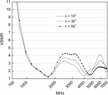
Figure 3.65 shows the simulation results of three antennas with different widths and heights. The three antennas have different widths and heights, which are 4 mm∗7 mm, 5 mm∗8 mm, and 6 mm∗9 mm respectively. All three antennas have the same length L = 30 mm, C-clip height = 3 mm, and θ = 30°. When the height and width of the antenna increase, the higher band performance does not significantly change while the lower band performance of the antenna improves. At 824 MHz, the VSWR of antennas with dimensions of 4 mm∗7 mm, 5 mm∗8 mm, and 6 mm∗9 mm is 10.3, 8.7, and 7.4 to 1, respectively. Based on these results, an antenna with dimensions of 5∗8 mm² is selected as a good compromise.

Shown in Figure 3.66 are the simulation results of four antennas with different antenna lengths. The antenna length varies from 25 mm to 40 mm. All four antennas have the same dimensions of H = 5 mm, W = 8 mm, C-clip height = 3 mm, and θ = 30°. As the antenna length increases, the VSWR of the antenna at the lower band improves significantly. At 824 MHz, the VSWR values of antennas of lengths 25 mm, 30 mm, 35 mm, and 40 mm are 12.9, 8.7, 6.2, and 4.6 to 1, respectively. It is observed that the higher band VSWR does degrade with the change in length, while the lower band's performance improves, as expected, with the length increase. As a compromise between industry design and antenna performance, a length of L = 30 mm is selected for the proposed design. It needs to be mentioned, when the L changes, the optimized θ might be different from 30°. The 30° is used here just to show the general trends.

A prototype antenna with following dimensions, H = 5 mm, W = 8 mm, L = 30 mm, C-clip height = 3 mm, and θ = 30°, was manufactured and tested. Generally speaking, the larger an antenna is the better the performance is at the lower frequencies. The lower band efficiency of an antenna is expected to improve with the increase in the antenna size.

Figure 3.67 shows the measured impedance of the prototype antenna before applying the matching network. The dashed line circle inside Figure 3.67 is the 3 : 1 VSWR circle. There are two markers that indicate the start frequency, 824 MHz, and the stop frequency, 6 GHz, of the desired operating band of the prototype antenna.

To match the lower band of a wide band antenna or a multi-band antenna, only two types of components can be used, which are shunt inductors and series capacitors. The order of those two components is decided by the impedance moving path on the Smith Chart, in this example a shunt inductor must be placed before a series capacitor if looking from the antenna side. Two extra matching components are used to improve the high band performance. When looking from the antenna side, the higher band matching networking includes, first, a 0.3 pF shunt capacitor and then a 1.0 nH series inductor. Figure 3.68a shows the final matching network implemented to achieve a VSWR better than 2.7 : 1 across the entire band. All four elements are 0402 (1 mm∗0.5 mm) surface mount chip components. Shown in Figure 3.68b is the impedance of the matched antenna. There is some measurement phase error (negative reactance slope) approaching 6 GHz. The reason is when the network analyzer was calibrated, it was calibrated to the SMA connector of the fixture pigtail instead of the matching circuit on the board. The standard port extension function of the network analyzer was used to simply shift the phase reference point to the matching circuit. That causes the larger phase error in the higher frequency band. To be more accurate, some means of calibration needs to be done instead of using the port extension method.

Figure 3.69 shows the measured VSWR data of the prototype antenna with the matching network. The measured VSWR is below 2.7 : 1 across the entire band. At the GSM850&900 (824∼960 MHz) band, the VSWR is below 2.1 : 1. At the 1575∼1675 MHz (GPS&DVB) band, the VSWR is below 2.0 : 1. At the 1710∼1990 MHz (DCS&PCS) band, the VSWR is below 1.8 : 1. At the 1920∼2175 MHz (UMTS) band, the VSWR is below 1.8 : 1. At the 2400∼2484 MHz (802.11b/g) band, the VSWR is below 2.5 : 1. At the 5150∼5875 MHz (802.11a) band, the VSWR is below 1.8 : 1.

Figure 3.70 shows the measured efficiency data. A Satimo® Stargate-64 3D near field chamber was used to measure the efficiency and patterns of the prototype antenna. The efficiency is defined as the ration of radiated power vs. total available power from power source. Thus, the efficiency value includes all the impacts from mismatch loss, dielectric loss, conductor loss, and matching component loss.

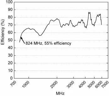
From the results shown in Figures 3.69 and 3.70, it may be noted that at the 824∼960 MHz band the efficiency is less than 65% when the VSWR values are better than 2.1 : 1. The lowest efficiency is actually 55% at 824 MHz and this is where the VSWR value is the highest without the matching network. If better than 55% efficiency is required, the highest VSWR without a matching network at the band edge of 824 MHz will have to be improved in the original design, say, by increasing the antenna height, width and/or length as demonstrated in Figures 3.65 and 3.66.

At the higher band, the overall efficiency is better than that at the lower band because the antenna VSWR at the higher band is quite low even without a matching network. From 1575 MHz to 6 GHz, an efficiency of 67∼88% was achieved. At the 1575∼1675 MHz (GPS&DVB-H US) band, the efficiency is 67∼72%, while at the 1710∼1990 MHz (DCS&PCS) band, the 1920∼2175 MHz (UMTS) band, the 2400∼2484 MHz (802.11b/g) band, and the 5150∼5875 MHz (802.11a) band, the efficiencies are 75∼79%, 70∼78%, 69∼72%, and 70∼83%, respectively.

Figure 3.71 shows the measured radiation patterns at 900 MHz and 5500 MHz. At 900 MHz, the antenna is similar to a dipole, which has a dominant polarized pattern E_θ. At higher frequency, because the current can be excited at both vertical and horizontal edges of PCB, the patterns are less polarized.

Shown in Figure 3.72 is a production UWB stubby antenna [23]. The only radiating part is the metal stamping. The snap finger, which is a mechanical feature to mate an antenna with a phone, is integrated with the plastic support. The contact feature is integrated with the metal stamping.

3.2 Whip-Stubby (Retractable) Antenna

We briefly discussed whip antennas in previous section and some comparisons between whip and stubby antennas have been given in Figures 3.1–3.20. In general, compared to a stubby antenna or an internal antenna, a whip antenna always has the widest bandwidth and the best performance. However, whip antennas are too cumbersome to be installed on most phone platforms, except on those phones that existed in the mid-1980s and had an appropriate nickname “brick.” To obtain the benefit of both stubby antennas and whip antennas, engineers invented the whip-stubby antenna, which is also called as retractable antenna. From the name, it is obvious that a whip-stubby antenna is a cross-breed between two different antennas. A whip-stubby usually has a retractable whip. When the whip is extended, because the whip is much longer than the stubby, it dominates the radiation and can achieve better performance. When the whip is retracted, the stubby becomes the primary radiator and the performance will degrade to a certain extent. Two different whip-stubby antennas are introduced in Sections 3.3.1 and 3.3.2 respectively. There are many more variants of whip-stubby antennas besides them. If using “retractable antenna” as the keywords, nearly 100 patents can be found in the US patent database.

3.2.1 Decoupled Whip-Stubby Antenna

The decoupled whip-stubby antenna is the most straightforward combination of a whip and a stubby. Figure 3.73 depicts such an antenna. The appearance and mechanical construction of decoupled antennas can vary significantly, however, they are all the same from the electrical point of view, as the whip and the stubby never work simultaneously. In Figure 3.73, all the transparent parts are made of plastic and all the solid parts are made of metal. The whole antenna assembly is composed of two independent radiators, a stubby in the top and a whip in the bottom. To ensure the electrical isolation between two radiators, the length of the plastic separator between radiators must be 5 mm or more. The metal whip is normally made of nickel-titanium alloy.

Figure 3.74 illustrates a decoupled antenna when it is installed on a phone. All the components inside the phone are omitted to better illustrate the antenna. Some mechanical features, such as the spring finger, the C-shape, or S-shape clip, are normally used to make an electrical connection between the metal connector and the feeding pad on a PCB. In Figure 3.74a, it is obvious that in the retracted position the whip is pulled all the way back and away from the metal connector inside the phone. The helix antenna is the only active radiator. In the extended position shown in Figure 3.74b, the whip makes connection with the metal connector and the helix is electrically floating on the tip of the whip. The whip is the only active radiator in this alternative position.

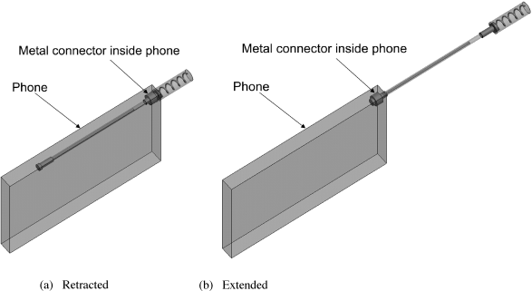
Designing a decoupled antenna is relative easy, because the two radiators are totally independent, so they can be tuned separately. However, because most phones only have one matching circuit, some extra attention needs to be paid to the design of both antenna and matching network.

The metal connector, which serves as the interface between an antenna and a circuit board, is the critical part in all whip-stubby antennas' design. To demonstrate the effect of the metal connector, two cases are simulated for comparison. Shown in Figure 3.75 are two whip antennas. In the first case as shown in Figure 3.75a, the whip is fed directly. In the second case as shown in Figure 3.75b, the whip is fed indirectly through a metal connector which is 10 mm long and 8 mm in diameter. Both whips are 80 mm long. Similar to the configuration shown in Figure 3.8a, a 70 mm∗120 mm metal board is used as the ground plane.

Shown in Figure 3.76 is the simulated reflection coefficients of both cases. It is clear that the metal connector slightly improves the lower band and significantly improves the higher band. Unlike stubby antennas, whips do not have too many tuning parameters besides the whip length and diameter. The length of a whip decides its lowest working frequency. Without the design freedom of metal connectors, we are probably stuck with the higher band response whatever a whip has. Fortunately, there are metal connectors to come to our assistance. Not a lot of skill is required to design a metal connector, larger is always better. As has been demonstrated in earlier sections, a metal connector can also improve the performance of stubby antennas.

3.2.2 Semi-Decoupled Whip-Stubby Antenna

Shown in Figure 3.77 is an example of a semi-decoupled whip-stubby antenna. All transparent parts are made of plastic and all solid parts are made of metal. All components inside the phone, including features to make the electrical connection between the metal connector and the feeding pad on a PCB, are omitted to better illustrate the antenna. The whole antenna assembly is composed of two radiators, a metal whip and a metal helix. The helix portion of the antenna is permanently attached to the phone. The whip can be extended and retracted. In the retracted position, as shown in Figure 3.77a, only the plastic part of whip sits inside the stubby and the metal whip is decoupled from the helix completely. In this position, the helix is the only active radiator. In the extended position, the whip extends all the way out of the phone and the end of whip slides into the metal connector. In this position, both the helix and the metal whip are electrically connected together, so both of them are activated.

From an electrical point of view, the design procedure of a semi-decoupled antenna is more complex than a decoupled one and its performance is a little worse. The merit of a semi-decoupled antenna is its robustness. As the stubby of a semi-decoupled antenna is permanently attached to the phone, the antenna assembly has better performance in drop tests and wear-out tests. Usually, the whip portion of an antenna is the weakest point in the whole structure. For a decoupled antenna, if the whip is broken, the antenna might get lost. For a semi-decoupled antenna, there is still a helix in the phone. Of course, different companies have different opinions on this matter, so some of them like decoupled solutions and the others like semi-coupled approaches.

In the retracted position, the helix of a semi-coupled antenna is the only active radiator. In the following example, the dimensions of the PCB, which functions as the ground, are 120 mm∗60 mm. The diameter and height of the metal connector are 8 mm and 10 mm respectively. The total height of the helix is 26 mm. The diameter of the helix is 7 mm. The pitch and number of turns of the helix are 4 mm and 6.5 respectively.

Shown in Figure 3.78 is the simulated response of the helix by itself. The thick solid lines in both figures illustrate the 824–894 MHz and 1850–1990 MHz, which are the presumed low and high bands. It is clear that the resonant frequency at low bands is offcentered, which is purposely designed.

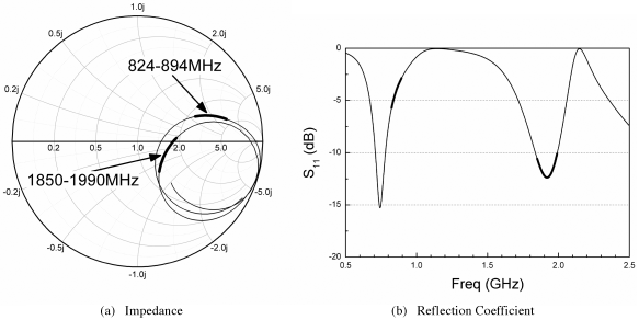
Shown in Figure 3.79 is the antenna's response when the whip is extended. The metal whip length is 90 mm if measuring from the top of the metal connector. Two narrow resonances, which are marked in both figures, are generated by the helix. As we have discussed in Figure 3.30, at these two frequencies there is strong current on the helix, however, it cannot effectively radiate due to the blocking effect of the center whip. As a result, the radiating efficiency at these frequencies is pretty low and needs to be avoided.

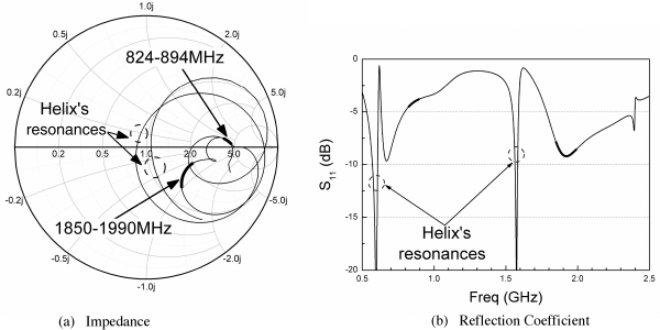
Shown in Figure 3.80 are the responses of a 90 mm whip by itself. Unlike Figures 3.78 and 3.79, the whip by itself is not a valid working state and the purpose of showing Figure 3.80 is to demonstrate the mutual impact between a whip and a helix. By comparing Figures 3.79 and 3.80, it is clear that due to the existence of the helix, the bandwidth of the whip is shrunk.

It might seem cumbersome to design a semi-coupled antenna, because so many elements are playing a role here. However, there is a programmatic design procedure which can be followed. When tuning a semi-coupled antenna, we have two goals. The primary goal is to adjust the impedances of both retracted and extended positions so they are in the same area on the Smith Chart. The location of the impedance at different bands can be different, as long as the impedances of the same band stay together. Then a matching circuit can be used to achieve a good impedance matching over all bands. If we tried to deal with the antenna's two positions separately, most likely it would be that whenever the antenna's performance in one position was tuned to the best, the performance in the other position would be significantly worse. To achieve a balanced performance, we must treat the impedance of both positions as a whole.

With the priority of the first goal, we still want to design the antenna to obtain a better matching, which is the secondary goal. Because the smaller an antenna's return loss is, the easier it is to design a matching circuit and the better its efficiency is. With the above two goals in mind, the actual design procedure has the following four steps:

• The first step is designing the whip. There is only one parameter, whip length, that can be adjusted. If a whip's basic resonant frequency is f₀, its next resonance is around 3∗ f₀. However, the ratio between the 850 MHz and 1900 MHz bands is about 2.2, so it is not practical to design a whip which intrinsically resonates at both bands. In the example shown in Figure 3.80, the whip is tuned at the high band, where its return loss is better than −8 dB. At the low band, the return loss is around −4 dB.
• The second step is designing the helix. A helix by itself corresponds to the antenna's retracted position. Our goal is to match the response of the helix to that of the whip at both bands. Techniques for designing a dual-pitch helix can be used to adjust the helix's response to the desired locations on the Smith Chart. In this example, a uniform helix is used. Because with the help of the metal connector, a uniform helix's response at both bands already meets our requirement, it is unnecessary to use a dual-pitch design.
• The third step is to put the helix and the whip together, fine tune them, then remove the whip, tune the helix alone, then tune both again. This step might take a few iterations. Some extra attention needs to be paid to those unwanted helix's resonances shown in Figure 3.79. The helix's resonances always move lower at the extended position. For a narrow band antenna, as in this example, no special treatment is needed, because the unwanted resonances will shift out of bands as shown in Figure 3.79. For a wideband antenna, the unwanted resonances might still be inside the low end of working bands. In this kind of circumstance, the helix's resonance must be tuned to a lower frequency and the whip length also needs to be tuned accordingly.
• The fourth step is to design a matching network. We must use the same circuit to match both the retracted and extended position simultaneously. This step is quite straightforward if the impedances of both positions are close enough on the Smith Chart.

Shown in Figure 3.81a is the four-element matching circuit of the final antenna. Shown in Figure 3.81b is the simulated reflection coefficients of both positions. The return losses of all bands at all positions meet the −10 dB specification. Beside the bandwidth of the low band in the retracted position, which is marginal, there is large margin in all other situations. The bandwidth in the extended position is more than twice as much as required. In practice, the specifications for retracted and extended position are often different. The performance of the extended position is more critical, because this is the normal usage position. In the meantime, the specification for the retracted position can be relaxed, because all users are aware that the whip should be extended if the call quality starts to degrade. If −6 dB is used as the specification for the retracted position, an antenna of the same dimension can cover penta-bands, 850 MHz, 900 MHz, DCS (1800 MHz), PCS (1900 MHz), and UMTS (2100 MHz), with some tweaks.

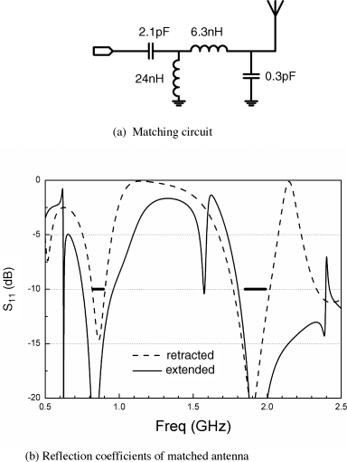
Shown in Figure 3.82 is a production retractable antenna. The antenna is a semi-decoupled whip-stubby. A dual pitch coil is used as the radiator when the antenna is in retracted position. In the extended position, a metal whip functions as the radiator. As the whip needs to be fully retracted into the phone, the total whip length must be less than its host's length. In this specific design, the phone's length is not long enough for the required band. A telescope tube is added to the design to provide the extra length. The whip slides in and out the telescope tube in the retracted and extended positions respectively.

3.3 Meander Line Stubby Antenna

With the progress of flex circuit technology, industry design engineers started to adopt the stubby antenna with the irregular cross-section. The radiator elements of some of those antennas are made of flex instead of coil. To accompany the flex, meander lines are introduced to replace the coil. The principle of a meander line antenna design is similar to a helix. Figure 3.83 demonstrates the transformation of a multiple branch meander line antenna.

When using the flex circuit technology, it is easier to implement multiple braches than use coils. Many variants of this type of antennas have been reported. Shown in Figure 3.84 is a dual band antenna for WLAN application [26]. Shown in Figure 3.85 is the simulated and measured reflection coefficients.

Shown in Figure 3.86 is another dual-branch multi-band monopole antenna [27]. Its simulated and measured reflection coefficients are shown in Figure 3.87. Although it may look like a single branch structure, the paths A and B are actually two independent branches.

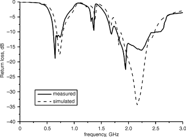
Shown in Figure 3.88 is a stubby antenna made of flex. The square pattern with a hole on the flex is the feeding point, which connects to a metal spring finger. A metal screw is used to secure the connection between them. Two traces come out of the feeding point. The short trace on the left side is for the high band and the longer one on the right is for the low band. Compared with a coil, a flex provides much more freedom on the trace layout. However, the basic rule still applies. Larger trace area means wider bandwidth. By diverting the available flex area to traces of different bands, the trade-off between bands can be made.

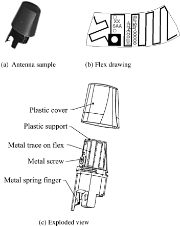
Shown in Figure 3.89 are some variants of multi-pitch meander line antennas. The left variant is quite straightforward. The right one is less conceivable. Both variants shown in Figure 3.89 are on a 2D surface. This type design can be extended to 3D surface.

Shown in Figure 3.90 is a multi-band antenna [28]. It is a 3D design and its design seems quite complex. However, this design is a combination of multi-branch and multi-pitch. This antenna gives a good demonstration of how much design freedom the flex technology introduces. Just remember, never over-design an antenna. An over-complex antenna will cause trouble in manufacturing and fine tuning later on.

The flex technology is also used in designs of retractable antennas. Shown in Figure 3.91 is a flex-based external antenna [29]. The antenna used a single-branch multi-band flex design. The flex design is similar to the whip-loaded helix antenna as shown in Figure 3.53. However, in a coil-based design, it is quite difficult to change the distance between the center whip and the coil. When adopting the flex technology, this parameter can easily be adjusted. Thus bandwidth between low and high band can also be easily exchanged.

3.4 Effect of Ground Plane

So far we have always accepted a ground as it is and then designed antennas around it. On the other hand, it has been demonstrated in Figure 3.8 that a ground isn't really a ground but one of the two radiation arms of an asymmetric dipole. Thus it should come as no surprise to know that the shape and size of a ground plane have prominent effects on the antenna built on it. Some published articles [30–33] have investigated the ground effect on a PIFA antenna or an IFA antenna. A straight wire monopole antenna is used here to study the effect. However, one should not count the dimension of a ground plane as a design freedom, because most of the time that dimension is solely decided by a product's industry design team. Some parameter studies presented here provide quantitative examples to help explain why some antennas work well on one phone but have problems when migrated to other phones. Other examples in this section illustrate some extreme cases when the ground is too small to function well.

The reason for using a monopole instead of a PIFA is to simplify the parameter studies. As shown in Figure 3.92, there are only three significant dimensions: monopole length L_ant, ground width W, and ground length L.

The antenna length, L_ant, used in all simulations shown in Figure 3.93 is 70 mm. In Figures 3.93a and b, the width of the ground plane, W, is 30 mm. The width is 70 mm for Figures 3.93c and d. For each ground width, three different ground lengths are compared.

In an asymmetric antenna, the resonant frequency is mostly decided by the smaller arm. The larger arm has a significant impact on the impedance, bandwidth and matching, but less effect on the frequency. In practice, sometimes it is quite tricky to decide which one is the short arm. As an example, the ground's length used in the simulation which generates the short dash curve shown in Figure 3.93b is 40 mm, which is shorter than the monopole's length 70 mm, but the ground cannot be considered the short arm. When a ground is small, its effective length can be approximated by the sum of two adjacent edges. In this case, the ground's effective length is the sum of 40 mm and 30 mm, which is about the same as the monopole. This can also be confirmed by Figure 3.93b. The resonant frequency of the monopole is 1.06 GHz, while a balance dipole with unilateral arm length of 70 mm resonates at 1.07 GHz.

The ground lengths of three curves in Figures 3.93a and b are 40 mm, 80 mm and 120 mm respectively. When the ground length increase, the antenna's response changes from single resonance to dual resonances. In the meantime, the impedance locus shifts toward the left side of the Smith Chart. It is obvious that a ground's length does have a significant impact on an antenna's response.

To illustrate the effect of the ground's width, all three cases shown in Figure 3.93a are simulated again with ground width increased to 70 mm. The results are shown in Figures 3.93c and d. It is clear that an antenna on a wider ground is less sensitive to the ground's length change.

The impact of ground on an antenna can be explained by the intrinsic modes of a ground itself. As shown in Figure 3.94a, 30 mm∗120 mm ground can support various mode at different frequencies. At 0.625 GHz, 120 mm equals to a quarter wavelength and the current on the board represents half a standing wave as shown in Figure 3.94a. In this figure, the size of arrows represents the current amplitude. To obtain the current distributions shown in all three figures, a 70 mm-long monopole is used to excite the ground. The square on the top-left corner is the feeding spot. The current on monopole antennas is omitted in all plots to conserve space. The current shown in Figure 3.94b represents one standing wave. In fact, at 1.25 GHz the current on the ground is composed of both a standing wave and a downward traveling wave. Figure 3.94b is a snapshot of the time-varying current distribution on the board. This snapshot illustrates the idea of current mode quite well. However, it is not an accurate representation of the actual board current at all times. At 1.875 GHz there is one and a half standing waves on the ground. Similar to the current at 1.25 GHz, there are both a standing wave and a downward traveling wave on the board.

When the ground becomes wider, a strong current can also be excited along the shorter edge. That spreads the current more evenly on the ground and thus makes the antenna's characteristic less sensitive to the ground length variation.

When an antenna is installed on a ground, the final antenna characteristic shows a combined effect of both elements. For example, a dipole with 70 mm unilateral arm length should resonate at 0.93 GHz. By combining a 70 mm-long monopole with a 120 mm-long ground, the antenna resonates at 0.78 GHz and 1.28 GHz respectively as shown in Figure 3.93b.

Besides impedance change, antennas' radiation patterns also vary when the ground's dimension is changed. Shown in Figure 3.95a is the radiation pattern of a 70 mm monopole when it is installed on a 30 mm∗40 mm ground. The radiation pattern is quite similar to the “donut” shape which is the trademark of a half-wavelength dipole antenna. The antenna can provide omni-directional coverage in the azimuth plane and also has its peak gain in that plane.

When fixing other parameters and only increasing the ground length from 40 mm to 120 mm, the antenna's pattern tilts downward as shown in Figure 3.95b. The tilting is due to the radiation of the downward traveling wave. The mathematical explanation can be found in many antenna books [25], the fact we need to remember here is the radiation pattern of a traveling wave structure always tilts toward the direction which the wave travels. In the case of monopole antennas, when the ground starts to be significantly larger than a quarter of a wavelength, a larger part of the current on the ground starts to take the form of a traveling wave, that tilts the radiation pattern down. On a cellular phone, it means an antenna's pattern at high frequency bands always tilts downward when the antenna is installed on the upper portion of the phone.

Shown in Figure 3.96 are the results of parameter studies of ground length. The monopole length is 30 mm and its approximate resonant frequency is 2 GHz. Three different board lengths, 40 mm, 80 mm, and 120 mm, are simulated. Shown in Figures 3.96a and b are results of narrow grounds, whose widths are 30 mm. Shown in Figures 3.96c and d are the results of 70 mm-wide grounds. Although the absolute ground dimensions used in Figure 3.96 are identical to Figure 3.95, the monopole length is different, thus the working frequency is different. At 2 GHz, the wavelength is less than half of that at 0.93 GHz, thus from the electrical point of view, the ground's relative dimension is more than doubled at 2 GHz. That explains why all the results shown in Figure 3.96 are less fluctuating. Comparing Figures 3.96b and d, it is clear that an antenna's impedance is less sensitive to ground length change when the working frequency is higher.

So far we have discussed the ground's impact on antennas' impedance when the ground grows bigger. Logically one will ask what will happen if a ground becomes smaller. Shown in Figure 3.97 are results of a 70 mm-long monopole antenna installed on three small grounds respectively. All three lines in Figure 3.97 illustrate responses of single resonance. With the ground becomes smaller, the resonant frequency shifts higher. One can shift the resonant lower by making the monopole longer, but only to a certain degree. It is quite difficult to achieve the required specification when designing a multi-band antenna on a small ground.

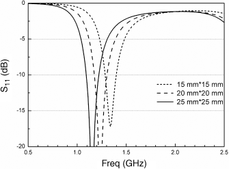
In summary, although antenna engineers do not have too much freedom in choosing a ground's dimension, we must be aware that the ground is one of the decisive factors influencing an antenna's bandwidth, radiation pattern and efficiency. Generally speaking, a larger ground is always better.

References

1. Iskander, M.F. (2000) Electromagnetic Fields and Waves, 1st edn, Waveland Press Inc.

2. Sadiku, M.O. (2009) Elements of Electromagnetics, 5th edn, Oxford University Press, USA.

3. Ulaby, F.T., Michielssen, E., and Ravaioli, U. (2010) Fundamentals of Applied Electromagnetics, 6th edn, Prentice Hall.

4. Buck, J. and Hayt, W. (2005) Engineering Electromagnetics, 7th edn, McGraw-Hill Science/Engineering/Math.

5. Moore, T.G., Borisov, E., Derdzinski, A., and Repplinger, D. (2002) Antenna assembly and multiband stubby antenna. US6369775B1.

6. Sutter, R.W., Weaver, W.B., and Dou, W. (2005) Multiple pitch antenna assembly. US6922178B2.

7. Zhinong, Ying (2000) Multi-band non-uniform helical antennas. US6112102.

8. The Federal Communications Commission of United States, First Report and Order, Revision of Part 15 of the Commission's Rule Regarding Ultra Wide Band Transmission Systems. http://hraunfoss.fcc.gov/edocs_public/attachmatch/FCC-02-48A1.pdf. Retrieved 25 October 2010.

9. Abbosh, A.M., Bialkowski, M.E., Mazierska, J., and Jacob, M.V. (2006) A planar UWB antenna with signal rejection capability in the 4–6 GHz band. IEEE Microwave and Wireless Components Letters, 16, 278–280.

10. Jianxin, L., Chiau, C.C., Chen, X., and Parini, C.G. (2005) Study of a printed circular disc monopole antenna for UWB systems. IEEE Transactions on Antennas and Propagation, 53, 3500–3504.

11. Kiminami, K., Hirata, A., and Shiozawa, T. (2004) Double-sided printed bow-tie antenna for UWB communications. IEEE Antennas and Wireless Propagation Letters, 3, 152–153.

12. Lin, C.C., Kan, Y.C., Kuo, L.C., and Chuang, H.R. (2005) A planar triangular monopole antenna for UWB communication. IEEE Microwave and Wireless Components Letters, 15, 624–626.

13. Low, Z.N., Cheong, J.H., and Law, C.L. (2005) Low-cost PCB antenna for UWB applications. IEEE Antennas and Wireless Propagation Letters, 4, 237–239.

14. See, T.S.P. and Ning, Chen Zhi (2008) An electromagnetically coupled UWB plate antenna. IEEE Transactions on Antennas and Propagation, 56, 1476–1479.

15. Verbiest, J.R. and Vandenbosch, G.A.E. (2006) Small-size planar triangular monopole antenna for UWB WBAN applications. Electronics Letters, 42, 566–567.

16. Verbiest, J.R. and Vandenbosch, G.A.E. (2006) A novel small-size printed tapered monopole antenna for UWB WBAN. IEEE Antennas and Wireless Propagation Letters, 5, 377–379.

17. Kian, Toh Wee, Ning, Chen Zhi, and Xianming, Qing (2009) A planar UWB antenna with a broadband feeding structure. IEEE Transactions on Antennas and Propagation, 57, 2172–2175.

18. Kian, Toh Wee, Ning, Chen Zhi, Xianming, Qing, and See, T. (2009) A planar UWB diversity antenna. IEEE Transactions on Antennas and Propagation, 57, 3467–3473.

19. Wong, K.L. and Chien, S.L. (2005) Wide-band cylindrical monopole antenna for mobile phone. IEEE Transactions on Antennas and Propagation, 53, 2756–2758.

20. Ni, Low Xue, Zhi Ning, Chen, and See, T.S.P. (2009) A UWB dipole antenna with enhanced impedance and gain performance. IEEE Transactions on Antennas and Propagation, 57, 2959–2966.

21. Jun, ChoYoung, Hak, Kim Ki, Hyuk, Choi Dong et al. (2006) A miniature UWB planar monopole antenna with 5-GHz band-rejection filter and the time-domain characteristics. IEEE Transactions on Antennas and Propagation, 54, 1453–1460.

22. Ren, Yu-Jiun and Chang, Kai (2006) An annual ring antenna for UWB communications. IEEE Antennas and Wireless Propagation Letters, 5, 274–276.

23. Zhang, Z., Langer, J.C., Sutter, R., and Kfoury, T. (2007) “Multiple band antenna and antenna assembly,” US7161538B2.

24. Zhang, Z. Langer, J.C., Li, K., and Iskander, M.F. (2008) Design of ultrawideband mobile phone stubby antenna (824 MHz–6GHz). IEEE Transactions on Antennas and Propagation, 56, 2107–2111.

25. Balanis, C.A. (2005) Antenna Theory: Analysis and Design, 3rd edn, Wiley-Interscience.

26. Khaleghi, A. (2007) Dual band meander line antenna for wireless LAN communication. IEEE Transactions on Antennas and Propagation, 55, 1004–1009.

27. Kim, S.C., Lee, S.H., and Kim, Y.S. (2008) Multi-band monopole antenna using meander structure for handheld terminals. Electronics Letters, 44, 331–332.

28. Kanj, H. and Ali, S.M. (2009) Compact multiband folded 3-D monopole antenna. IEEE Antennas and Wireless Propagation Letters, 8, 185–188.

29. Kfoury, T. and Mathews, J. (2006) Clipped contact whip and flex antenna assembly for a device. US7095375.

30. Arkko, A.T. (2003) Effect of ground plane size on the free-space performance of a mobile handset PIFA antenna. Twelfth International Conference on Antennas and Propagation, 2003. (ICAP 2003). (Conf. Publ. No. 491). vol. 1, pp. 316– 319.

31. Chan, K.H., Fung, L.C., Leung, S.W., and Siu, Y.M. (2006) Effect of internal patch antenna ground plane on SAR. 17th International Zurich Symposium on Electromagnetic Compatibility, 2006. EMC-Zurich 2006, pp. 513– 516.

32. Fujio, S. (2006) Effect of ground size on plate inverted-F antenna. International Workshop on Antenna Technology Small Antennas and Novel Metamaterials, 2006 IEEE, pp. 269– 272.

33. Urban, R. and Peixeiro, C. (2004) Ground plane size effects on a microstrip patch antenna for small handsets. 15th International Conference onMicrowaves, Radar and Wireless Communications, 2004. MIKON-2004, vol. 2, pp. 521– 524.