
11. Creating Charts and Sparklines
In This Chapter
• Quickly add a chart to a sheet.
• Create a chart mixing bars and lines.
• Make a pie chart easier to read.
• Insert sparklines into a report.
Charts are a great way to graphically portray data. They’re a quick and simple way to emphasize trends in data. Some people prefer to look at them instead of trying to make sense of rows and columns of numbers. Excel offers two methods of charting data—charts and sparklines. Charts, which you are most likely familiar with, are large graphics with a title and numbers and/or text along the left and bottom. Sparklines are miniature charts in cells with only markers to represent the data. This chapter provides you with the tools to create simple, but useful, charts. For further information, refer to Charts & Graphs: Microsoft Excel 2013 (ISBN 978-0-7897-4862-1) by Bill Jelen.
Preparing Data
The first step in creating a chart is ensuring that the data is set up properly. Although the following rules aren’t going to prevent a chart from being created, heeding these rules allows Excel to help you create a chart by identifying the chart components:
• Ensure that there are no blank rows or columns.
• Ensure that headers along the left column and top row identify each series.
• If your row or column headers include numbers, leave the upper-left corner of the chart blank (see cell A1 in Figure 11.1). If the cell isn’t blank, Excel may be confused when it tries to help you create the chart and it may assume there are no category labels and chart the header as data.
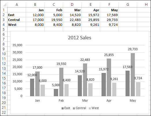
Figure 11.1. A basic chart and its source data. A chart consists of many components that you can configure.
Elements of a Chart
A chart is a graphical representation of numerical data. Behind every chart is a data range on a sheet, like the table shown in A1:F4 in Figure 11.1. This range is called the source data.
A series is a row or column from the source data represented on the chart as a line, a bar, or other marker used to portray the data. A typical series consists of the following:
• Series name—The cell with the name of the series that will appear in the legend
• Series values—The row or column containing the data to be charted
• Category labels—The range containing the label that will appear along the axis, identifying the series value
In Figure 11.1, the series names are East, Central, and West. The series values are presented by the thick-shaded vertical columns. The category labels are the months, Jan through May, along the horizontal axis, also known as the x-axis.
 Note
Note
If using the Quick Analysis tool or Recommended Charts options, Excel will help you create a chart by trying to ascertain whether the rows or columns in the source data are to be used as a series. Normally, the row or column set consisting of fewer items will default to the series, but Excel may switch this depending on the chart type. If the number of rows and columns are equal, Excel may offer a chart of each type. In Figure 11.1, Excel correctly determined that East, Central, and West were the series for the chart because the source data had fewer rows (three) than columns (five).
 Caution
The following chart elements are the most common. Not all may appear depending on the selected chart’s type.
Gridlines are horizontal or vertical lines in the chart that help make it easier to read the values of the markers.
The axes consist of major and minor gridlines that usually go below and to the left of the charted data (except for pie charts), labeling or marking intervals of the data. An axis may also have an Axis Title or Display Units Label. The horizontal axis, the one that goes left to right, is also known as the x-axis. The vertical axis, the one that goes up and down, is also known as the y-axis.
The legend is the color code for the chart series, identifying each series by the name assigned to it. In Figure 11.1, the legend is placed along the bottom of the chart.
Data labels are text that appears in the chart by the series marker, identifying the value of the points being charted, as shown in Figure 11.1.
The chart title is located at the top of the chart. By default, it isn’t linked to a cell on the sheet—you must manually type it in.
See the section “Editing and Formatting a Chart Title” for a tip on linking a chart title to a cell.
Error bars are markers on a chart that look like the capital letter I. They’re used to see margins of error in the data.
A trendline is a line on a chart that shows data trends, including future values. Trendlines can only be added to the following nonstacked, 2D charts: bar, column, line, area, stock, and scatter.
Put together, a chart has two areas:
• Plot area—Consists of the series and inner gridlines
• Chart area—Consists of the area surrounding the plot area, including the frame of the chart
Types of Charts
There are ten chart groups, each with several types you can select from, in Excel. Further manual changes, such as mixing chart types, provide even more variations. The ten charts groups are:
 Tip
Tip
In the Charts group on the Insert tab, there are eight buttons, with the Radar drop-down button listing Stock, Surface, and Radar.
• Column—Includes 2D Column and 3D Column chart types that feature markers relating the vertical height to size. They are useful for showing data changes over a period of time or comparing items. 3D Cylinder, 3D Cone, and 3D Pyramid charts can be created by modifying a 3D Column chart.
• Line—Includes 2D Line and 3D Line chart types. They are useful for displaying continuous data over time against a common scale.
• Pie—Includes 2D Pie, 3D Pie, and Doughnut chart types. Pie charts are most suitable for single-series data sets. They are useful for showing how an item is proportional to the sum of all items. A doughnut chart is similar to a pie chart in that it shows how an item is proportional to the whole, but unlike a pie chart, it can include more than one series.
• Bar—Includes 2D Bar and 3D Bar chart types that feature markers relating the horizontal width to size. They are useful for comparing items. 3D Cylinder, 3D Cone, and 3D Pyramid charts can be created by modifying a 3D Column chart.
• Area—Includes 2D Area and 3D Area chart types. They are similar to line charts except that the area underneath the line is filled with color. Area charts emphasize the magnitude of change over time.
• Scatter (XY)—Includes Scatter chart types of just markers, just lines, or combined markers and lines. They show the relationships among numeric values in several data series or can be used to plot two groups of numbers as one series of x,y coordinate. Also includes 2D Bubble and 3D Bubble chart types used to plot data points with the size of a bubble suggesting its relationship to the other bubbles.
• Stock—Illustrates the fluctuation of the data, such as stocks or temperatures.
• Surface—Finds the optimum combinations between two sets of data.
• Radar—Compares the total values of several data series.
• Combo—Helps you combine multiple chart types. See the section “Creating a Chart with Multiple Chart Types” for more information.
Column, Line, Bar, and Area chart types have three basic patterns available:
• Clustered—In a clustered chart, the markers are plotted side by side, making it easier to compare markers. The downside is that it is more difficult to tell if the data is increasing or decreasing in comparison with the next cluster. When viewing the chart types, clustered chart types show a light marker next to a dark marker.
• Stacked—In a stacked chart, the markers are plotted on top of each other, making it easier to see how the sum of data changes, but making it more difficult to see how a specific series changes over time. When viewing the chart types, stacked charts show a dark marker on top of or to the right of a light marker. The stacks are of differing heights.
• 100% stacked—In a 100% stacked chart, the markers are plotted on top of each other. All stacks are scaled to have a height of 100%, allowing you to see which data points make the largest percentage of each stack. When viewing the chart types, stacked charts show a dark marker on top of or to the right of a light marker. The stacks are of the same heights.
Caution
With the variety of charts available and the settings to make them eye catching, you might be tempted to choose a chart type based on its visual appeal—but keep in mind that not all chart designs will properly convey a true interpretation of the data. For example, look at the chart in Figure 11.2. A 3D pyramid is a fun way of looking at data, especially during a long presentation. But compare the three sections—do they really tell the truth of the data? The value of the base of the pyramid is less than half of the top value. But that is difficult to tell from just the image. Imagine if the data values weren’t turned on? And compare the middle section with the top. They look about the same, with perhaps the middle slightly larger, but the data values tell a different story.
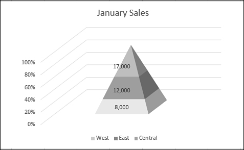
Figure 11.2. A bad chart design can distort the truth about the data.
Adding a Chart to a Sheet
There are three ways to add a chart to a sheet. With two of the methods—Quick Analysis tool and Recommended Charts—you pick from a group of charts Excel has selected for you. You can still customize the chart after it’s placed on the sheet—Excel just offers a place to start. The third method allows you to choose from all available charts.
Once you’ve added a chart to a sheet, you can select it by clicking anywhere in the chart area. No matter which method you choose, you’ll have to add a chart title after the chart is inserted. See the section “Editing and Formatting a Chart Title” for instructions on how to do this. You’ll also be able to change the color and apply a chart style (see the section “Applying Chart Styles and Colors”).
Using the Quick Analysis Tool
The Quick Analysis tool is a quick way to insert a chart on a sheet. When you select data on the sheet, the Quick Analysis tool appears in the lower-right corner of the selection, as shown in Figure 11.3. When you click on the icon and select Charts, Excel suggests different chart types based on its analysis of the selected data. Although the data in Figures 11.3 and 11.4 is the same, the selections differ and Excel’s chart type recommendations differ, too.
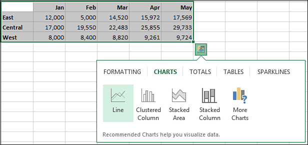
Figure 11.3. Use the Quick Analysis tool to bring up a list of suggested chart types.
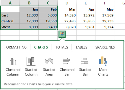
Figure 11.4. The list of suggested chart types will change depending on the selected data.
As you move your cursor over the suggestions, a preview image appears, so you can see what your data would look like in the selected chart type. When you’ve decided which chart you want, click on the icon and Excel inserts the chart on the sheet. If you don’t see a chart type you like, selecting More Charts opens up a list of the Recommended Charts. See the following section “Viewing Recommended Charts.”
Viewing Recommended Charts
You don’t have to select your data range before viewing Excel’s recommended charts, but it does ensure that Excel properly interprets the range. You must have at least one cell in the source data selected, then go to Insert, Charts, Recommended Charts and the Insert Chart dialog box shown in Figure 11.5 opens.
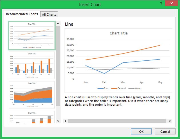
Figure 11.5. Excel recommends charts based on its interpretation of your data.
On the left side of the dialog box are Excel’s recommended charts. Click on a chart and a larger version appears on the right side of the dialog box. When you see one you like, select it and then click OK. It is added to the active sheet. If you don’t see a chart type you like, select the All Charts tab to see all the charts available in Excel. See the following section “Viewing All Available Charts” for more information.
Viewing All Available Charts
For access to all available charts—not just the ones Excel thinks you might find useful—select at least one cell in your source data and then select one of the chart type drop-downs in the Charts group of the Insert tab or click on the See All Charts dialog launcher in the lower-right corner of the Charts group.
If you open a drop-down from the Charts group, you can move your cursor over the individual charts and a preview appears on the sheet. If you see the chart you want, click on its icon and the chart is added to the sheet.
If you don’t see the chart you want, select the More [chart type] Charts text at the bottom of the drop-down to open the Insert Chart dialog box to the chart group you were looking at previously. If you click the ribbon shortcut instead, it opens the Insert Chart dialog box to the Recommended Charts tab. Click the All Charts tab to view all charts.
The left side of the Insert Chart, All Charts dialog box, shown in Figure 11.6, lists all the chart groups available. When you select a group, the available types are shown along the upper-right side of the dialog box. If you select a type, a preview appears below the types. Depending on the source data setup, you might get two or more previews, reflecting possible data series configurations. If Excel cannot interpret the source data, you don’t get a preview image. For example, an Open-High-Low-Close Stock chart requires a very specific setup of opening price, high price, low price, closing price.
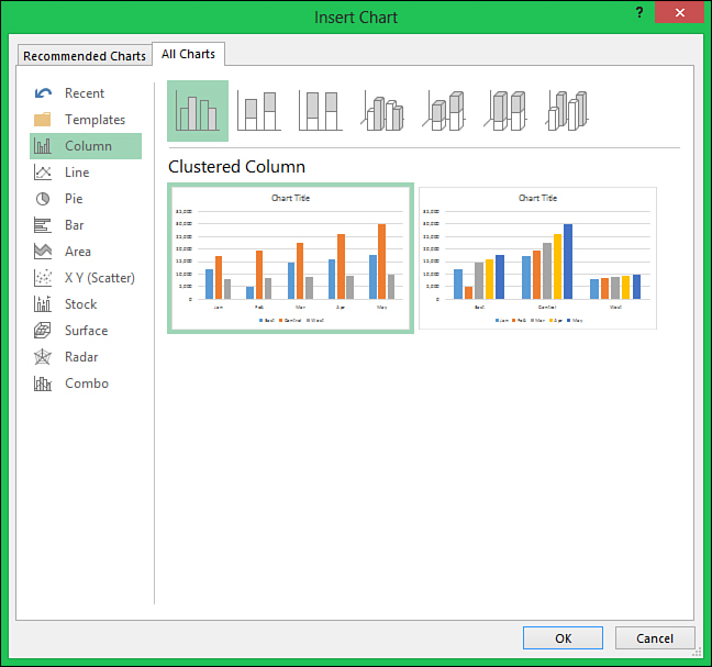
Figure 11.6. Choose from all the charts Excel has to offer through the All Charts option.
When you place your cursor over a preview, a larger version appears. Once you find the chart you want, select it, and then click OK; it is added to the sheet.
Adding, Removing, and Formatting Chart Elements
When you select a chart, three icons appear on the right side of it. The first, which looks like a plus sign, is for Chart Elements, the items reviewed in the section “Elements of a Chart.”
Note
You can also access a list of elements by going to Chart Tools, Design, Chart Layouts, and opening the Add Chart Elements drop-down. This list doesn’t offer the ability to turn elements on/off by just selecting the element. Instead, you must open the element’s submenu and make a selection.
Select an element to have it appear in the chart. Deselect it to hide it. For additional options concerning the element, such as its location in the chart, click on the arrow that appears to the right of the element. A list of options appears, as shown in Figure 11.7. Selecting More Options opens a task pane on the right side of Excel. Depending on the selected element, the options shown change, but it is from this task pane that you can make more changes to the element’s formatting, such as the color, 3D design, and alignment.

Figure 11.7. The Chart Elements list allows you to turn an element on or off and adjust its settings.
Editing and Formatting a Chart Title
Unless you have a single data series with a row header, when you insert a chart, Excel places a “Chart Title” placeholder at the top of the chart. To change the text, click in the text box and replace the generic “Chart Title.” You can also apply formatting to the title. If you select the entire text box, the formatting will apply to the entire title. Else, you can select a single character or word and format just that.
Caution
The selection frame around the text box changes depending on the mode the selection is in. When the frame is selected and the frame is solid, any formatting will apply to the entire frame and its contents. If the frame is dashed, then the selection is inside the frame.
Tip
To move the text box to a custom location, place your cursor along the box edge until it turns into a four-headed arrow. At this point, hold down the mouse button and drag the box to a new location.
Excel doesn’t have the built-in ability, but with a little work, you can create a dynamic chart title linked to a cell. To do this, select the title text box, ensuring the selection frame is solid, not dashed. Next, place your cursor in the formula bar, type an equal sign (=), and then click on the cell containing the title text. Press Enter and the title updates to reflect the cell’s text. As the text in the cell changes, the chart title also updates.
If you decide to make the title static again, right-click on the title and select Edit Text. You can also toggle the chart title on and off to reset the title.
Changing the Display Units in an Axis
Excel bases the units shown in an axis off the data. Excel displays units in millions or billions if that is what your data contains, taking up quite a bit of room. You can change the display units, reducing the amount of space used and making the axis easier to read. To do this, right-click on the axis and select Format Axis. From the task pane, select Axis Options, the last icon that looks like a chart. Near the bottom of the Axis Options section is a section for Display Units, as shown in Figure 11.8. Open the drop-down and select how you want the units abbreviated. If you don’t want abbreviation text appearing by the axis, deselect Show Display Units Label on Chart. Instead, you can customize the chart title, as shown in Figure 11.8.
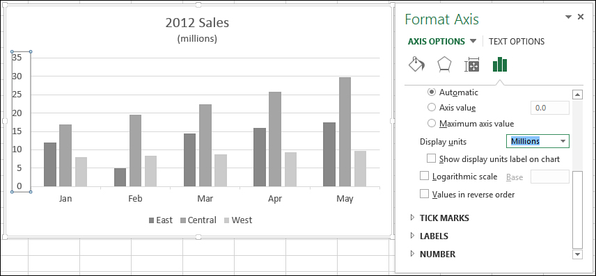
Figure 11.8. Change the display units of a numerical axis to reduce the amount of space used.
Applying Chart Styles and Colors
Once you’ve inserted a chart, you may want to move the chart title, move the legend, add a background, change the color of the series, or apply any number of changes to make the chart more attention getting. You can apply each change yourself, or you can see what chart styles Excel has available.
When you select a chart, three icons appear along the right side of it. Clicking the second icon with the paintbrush opens up a Style dialog box, in which you can scroll and view various styles, as shown in Figure 11.9. As you place your cursor over each one, your chart updates and provides a preview of the style. When you find a style you like, click it and your chart will update.
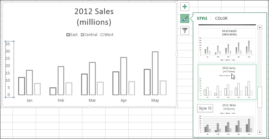
Figure 11.9. Apply one of Excel’s existing chart styles to create an eye-catching chart.
Note
You can also access this list of styles by selecting your chart and going to Chart Tools, Design, Chart Styles.
If you click the Color tab of the Styles dialog box (or go to Chart Tools, Design, Change Colors), various color combinations are shown. If you place your cursor over a color sample, the data series in the chart updates. When you find a color scheme you like, click it and your chart updates.
Tip
If you click once on a single series in the chart so that only the series is selected, then go to Chart Tools, Format, Shape Styles, Shape Fill, you can change the color of the selected series. If you click twice (two single clicks, not a double-click) on a specific data point in a series so that only it, not the entire series, is selected, you can apply a color to just that data point.
Applying Chart Layouts
Chart layouts are predefined layouts offering combinations of the chart elements: legend, chart title, axis title, data labels, and data table. From Chart Tools, Design, Chart Layouts, Quick Layout, up to 12 layouts are available, depending on the type of chart selected. If you place your cursor over a layout sample, the chart updates and provides a preview. When you find a layout you like, click it and your chart updates. If none of the predefined combinations is what you want, you can manually modify each element.
Moving or Resizing a Chart
The default location for a chart is the same sheet as the data. If you create your chart using the Quick Analysis tool or the Recommended Charts options, you have no control on where the chart is initially placed. But a chart can be moved to another location on the same sheet, to a new sheet, or to its own chart sheet.
To move a chart elsewhere on the same sheet, click anywhere in the chart area and drag the chart to the new location. Be careful not to click in the plot area or you’ll move the actual chart itself within the frame.
To relocate the chart to another sheet, first make sure the new sheet exists. Then, select the chart and go to Chart Tools, Design, Location, Move Chart. From the Move Chart dialog box that opens, select the new sheet from the Object In drop-down.
A chart sheet is a special type of sheet in Excel used to display only charts. It doesn’t have cells like the other sheets and you can’t add any information to it, other than the chart components. To relocate the chart to its own chart sheet, select the chart and go to Chart Tools, Design, Location, Move Chart. From the Move Chart dialog box that opens, select the New Sheet option. Charts on a chart sheet cannot be resized, except by zooming in and out on the sheet.
To resize a selected chart, place the cursor at any of the four corners or midway along any of the edges of the frame. When the cursor changes to a double-headed arrow, click and drag the chart to the desired size.
Switching Rows and Columns
If, after inserting a chart, you want to switch the row/column setup being used for the data series, select the chart and then click the Switch Row/Column button found on the Chart Tools, Design tab in the Data group. Excel switches the range used for the series and the range used for the category labels.
Changing an Existing Chart’s Type
You don’t have to re-create a chart from scratch if you want to change the chart type. Just select the chart; go to Insert, Charts; and select a new chart type from the drop-downs. Any formatting that can transfer over will be included in the new chart type. You can also go to Chart Tools, Design, Type, Change Chart Type. See the section “Viewing All Available Charts” for instructions on using the dialog box.
Creating a Chart with Multiple Chart Types
Some of the chart types can be used together in a single chart, as shown in Figure 11.10, where region series are column charts and the monthly average a line chart. You can do this by selecting Combo as the chart type. If you need to change an existing chart into a combo chart, see the preceding section, “Changing an Existing Chart’s Type.”
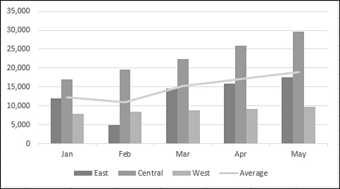
Figure 11.10. Use a combo chart to add a line to show how each region compares with the average.
Tip
Excel does not show a combo chart as a recommendation when you select from the Quick Analysis tool or Recommended Charts. You must insert the chart using the instructions in the section “Viewing All Available Charts.”
Select Combo from the Insert Chart or Change Chart Type dialog box and Excel provides a few predesigned combo charts to choose from. If none of the options is what you want, click the last icon, Custom Combination, which looks like a pencil over a column chart. At the bottom of the dialog box, shown in Figure 11.11, each series has its own line, which shows the series name, chart type, and whether the series should be shown on a secondary axis. As you select different chart types, the preview window updates. Once you have the chart types you want, click OK.
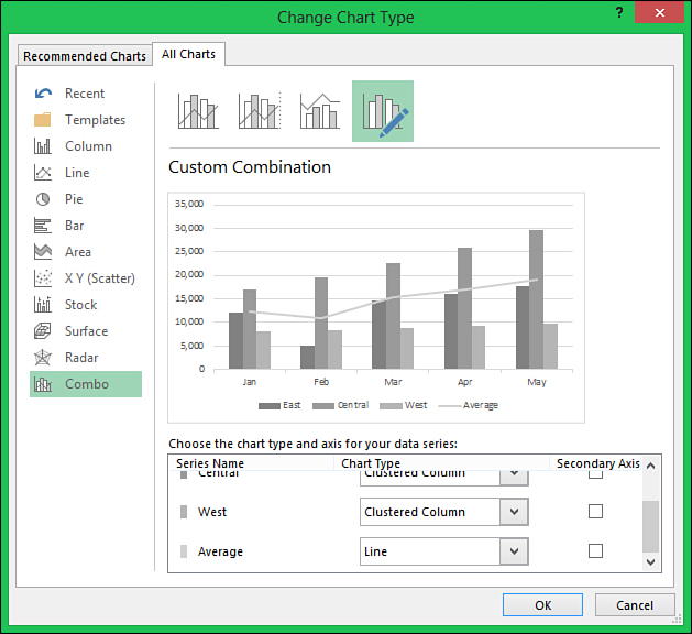
Figure 11.11. You can mix a variety of chart types using the Combo chart type.
A secondary axis is an axis that appears on the right side of the chart. It is often used for charting data of a different scale. For example, if you’re charting dollars and percentages, you could have the dollar data attached to the left axis and the percentages attached to the right axis.
Updating Chart Data
Unless the source data is a Table, the chart won’t automatically update as new data is added to the data set. To manually update the data source of a chart, do one of the following:
• Go to Chart Tools, Design, Data, Select Data, or right-click the chart and choose Select Data. Update the Chart data range in the Select Data Source dialog box, shown in Figure 11.12.
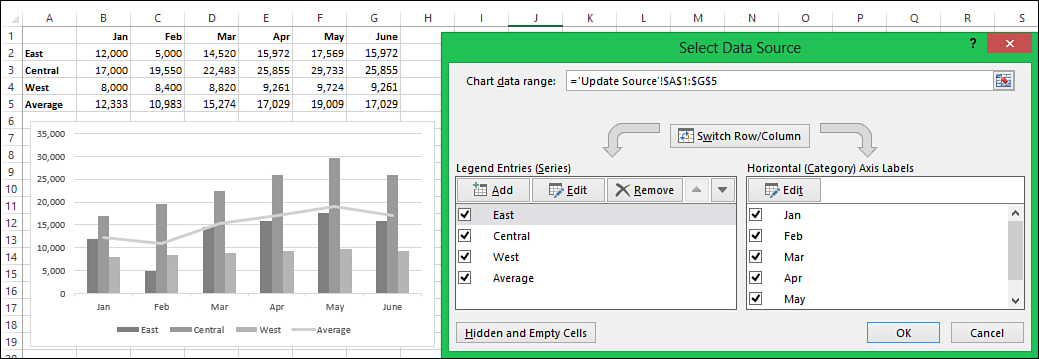
Figure 11.12. The original data range was A1:F5. After adding the June data, the source data range is updated to include the new data in the chart.
• When the chart is selected, the data source is highlighted with a colored border. The borders can be manually modified, changing the source range, by clicking and dragging to include the new rows. Make sure you place your cursor in the corner of the range and get a two-headed arrow, not a four-headed arrow. If using this method, be careful to not move the range when trying to expand it.
In addition to the two previous methods, the existing series on a chart can be updated by copying the new data and pasting it into the chart. To do this, follow these steps:
1. Ensure that the new data has a header similar to the existing data. It is especially important that a heading entered as a Date is still a Date and not Text.
2. Select the new data, including the header.
3. Right-click over the selection and choose Copy.
4. Select the chart.
5. Go to Home, Clipboard, Paste. The chart updates with the new data.
Creating Stock Charts
There are four types of stock charts that you can create using historical stock data. Each type has specific requirements for included columns and their order. If the order of the data is not met, the chart will not be created. The charts and their required columns and order are as follows:
• High-Low-Close—Requires four columns of data: Date, High, Low, Close
• Open-High-Low-Close—Requires five columns of data: Date, Open, High, Low, Close
• Volume-High-Low-Close—Requires five columns of data: Date, Volume, High, Low, Close
• Volume-Open-High-Low-Close—Requires six columns of data: Date, Volume, Open, High, Low, Close
After the data is in the correct column order, the chart can be selected from the Other Charts drop-down. See “Viewing All Available Charts” for inserting a stock chart.
Tip
Excel doesn’t read the column labels to determine if you have set up your data correctly. It can only count the number of columns in the data source. So make sure the data source includes only the columns for the desired stock chart, not including a Date or Stock Name column.
Creating Bubble Charts
You may want to use a bubble chart because they are unusual, but there is also a practical reason for using one. With a bubble chart, you can display a relationship among three variables. The x,y coordinate represents two variables, and the size of the bubble is the third.
In Figure 11.13, Age and Miles are charted along the x- and y-axes, respectively. The Price becomes the size of the bubble at the intersection of the x,y coordinate. See “Viewing All Available Charts” for inserting a bubble chart.
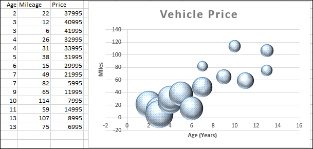
Figure 11.13. The size of the bubble at the intersection of the x- and y-axes represents the relative price of the vehicle.
Pie Chart Issue: Small Slices
When creating a pie chart, you may end up with slices that are very difficult to see. Two possible ways of dealing with this are to rotate the pie or create a bar of pie chart.
Rotating the Pie
Rotating the pie works best if the chart is 3D. By rotating the chart so the smaller slices are toward the front, they are easier to see, as shown in Figure 11.14. To rotate the pie, follow these steps:
1. Select the chart by clicking along the chart’s frame.
2. Go to Chart Tools, Format, Current Selection, and select the series from the Chart Elements drop-down.
3. Select Format Selection.
4. From the Series Options category (the far-right icon that looks like a column chart), move the Angle of First Slice slider to the right. The chart updates when you let go of the mouse button, so you can see how far you need to move the slider.
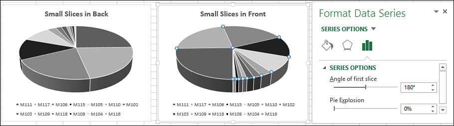
Figure 11.14. Rotate the pie chart to place the smaller pie slices toward the front, making them easier to see.
Creating a Bar of Pie Chart
Bar of Pie is one of the options listed under Pie (see “Viewing All Available Charts”). It’s used to explode out the smaller pie slices into a stacked bar chart, as shown in Figure 11.15, making the smaller slices more visible. Excel will create a new slice called Other, which is a grouping of the slices now in the bar. But the default explosion might not be adequate to your needs—you might want to include more smaller pieces in the bar chart. You can include more pieces by going into the Format Data Series task pane and changing the number of values included in the bar.
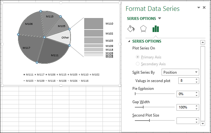
Figure 11.15. Use a bar of pie chart to group smaller slices into a stacked bar chart, making the smaller slices more visible.
To change an existing pie chart to a bar of pie chart and modify the number of slices used in the stacked bar in the chart, follow these steps:
1. Select the pie chart.
2. Go to Chart Tools, Design, Type, Change Chart Type.
3. In the Change Chart Type dialog box, select Bar of Pie from the Pie options.
4. Click OK. The chart changes to a bar of pie chart. If you’re happy with the default selection for the number of slices moved to the stacked bar, you’re done. Otherwise, continue to step 5 to change the number of slices used in the bar.
5. With the chart still selected, go to Chart Tools, Format, Current Selection, and select the series from the Chart Elements drop-down.
6. Click Format Selection. The Format Data Series task pane opens.
7. From the Series Options category, change the number of Values in the Second Plot field. As the value is changed using the spin buttons, the chart updates.
8. When satisfied with the chart, click Close.
Tip
Adjust the size of the bar chart by changing the Second Plot Size value in the Format Data Series task pane.
Adding Sparklines to Data
A sparkline is a chart inside of a single cell based on a single row or column of data. It can be placed right next to the data it’s charting or on another sheet. Because the sparkline is in the background of the cell, you can still enter text in that cell.
There are three types of sparklines available: Line, Column, and Win/Loss. Different colors can be applied to them, and various settings in the Show group of the Sparkline Tools, Design tab affect how the sparkline will be designed.
To add a sparkline to your data, select either the cell where you want the sparkline to go or the data set (not including the headers) and go to Insert, Sparklines. Fill in the fields of the Create Sparklines dialog box and the sparklines are added to the selected location.
As long as Excel can tell you have the same number of sparkline cells and corresponding ranges, you can create adjacent sparklines based on adjacent data sets. Just select the multiple sparkline cells or data sets at the same time. If you create sparklines together using this method, they will be grouped, and changes to the settings will affect them all.
Adding Points to a Sparkline
After you’ve created a sparkline, you can choose to show the High Point, Low Point, Negative Points, First Point, Last Point, and Markers (line charts only), as shown in the first three examples in Figure 11.16. To add points to a sparkline, select the sparkline and go to Sparkline Tools, Design, Show, and select the desired points. Each point can be assigned its own color by going to the Marker Color drop-down in the Style group of the tab. For example, to create the first set of sparklines in Figure 11.16, follow these steps:
1. Select F3:F5, the cells where the sparklines will be placed.
2. Go to Insert, Sparklines and select Column.
3. Place your cursor in the Data Range field, and then select range B3:E5 on the sheet.
4. Verify the Location Range is correct, and then click OK.
5. From the Show group on the Sparkline Tools, Design tab, select High Point. Excel colors the high point in each sparkline a different color.
6. To change the color of the high point, go to the Marker Color drop-down in the Style group. From the drop-down, select High Point, and then select a new color for the marker.
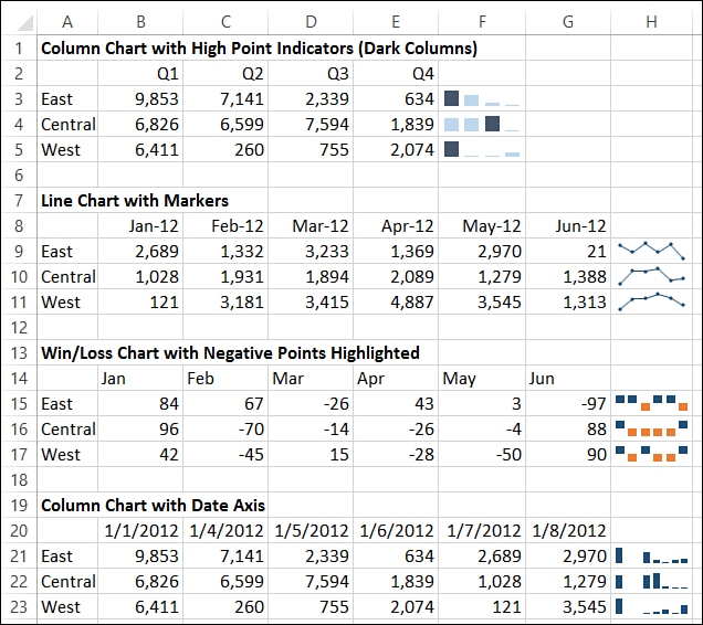
Figure 11.16. Use Sparklines to add in-cell charts to your data.
Spacing Markers in a Sparkline
The fourth set of charts in Figure 11.16 uses the Date Axis Type option to space the columns out in respect to the date of the data set. Note the space in the sparkline between the first and second columns. This is parallel to the date difference between the first two columns of data. The setting is available in the sparklines Axis drop-down in the Group group.
The date range must include real dates. For example, Jan, Feb, Mar, and the like won’t work because these are not actual dates, but if the actual dates are 1/1/12, 2/1/12, 3/1/12 and they are simply formatted to just show the month, they will work to space out the data in the sparkline.
To space out sparklines based on the dates in the data set, as shown in Figure 11.16 where there are two days (1/2/12 and 1/3/12) missing between the first and second dates, follow these steps:
1. Select a cell in the sparkline group.
2. Go to Sparkline Tools, Design, Group, Axis, and select Date Axis Type from the drop-down.
3. The Sparkline Date Range dialog box opens. Select the date range, B20:G20 in Figure 11.16, to apply to the sparklines.
4. Click OK. The sparklines update to accommodate the spacing in the selected date range.
Deleting Sparklines
You cannot simply highlight a sparkline and delete it. Instead, to delete a sparkline, go to Sparkline Tools, Design, Group, Clear, and choose either Clear Selected Sparklines to clear just the selected sparkline or Clear Selected Sparkline Groups, to clear a set of sparklines grouped together.
Creating a Chart Using a User-Created Template
If you have a chart design you want to apply to multiple charts, you can save the design as a template. All the settings for colors, fonts, effects, and chart elements are saved and can be applied to other charts. Because the template is saved as an external file, you can share it with other users.
To create the template, build and customize a chart. Then right-click on the chart and select Save as Template. Give the template a name and click Save. The template is now available in the Templates option of the Insert Chart dialog box and can be applied just like the Excel-defined charts.
Caution
You must use the default location for saving charts so the chart will appear in the Insert Chart dialog box.
Tip
If you receive a chart template, save it to the following folder:
\AppdataRoamingMicrosoftTemplatesCharts
Any templates saved to this location appear in the Insert Chart dialog box.