
Parallel programming illustrated through Conway’s Game of Life
Victor Eijkhout* * The University of Texas at Austin
Abstract
This chapter introduces a number of basic concepts in parallel programming using the Game of Life as an example. No specific programming systems will be taught here, but this chapter should leave the student with a basic understanding of the fundamental concepts. There are some pen-and-paper exercises.
Relevant core courses: The student is supposed to have gone through CS1, with CS2 and DS/A preferred.
National Science Foundation/IEEE Computer Society Technical Committee on Parallel Processing curriculum topics: All topics have a Bloom classification of C unless otherwise noted.
Architecture topics
• Taxonomy: single instruction, multiple data (Section 10.2.1); multiple instruction, multiple data/single program, multiple data (Section 10.2.3)
• Pipelines: Section 10.2.1
• Dataflow: Section 10.2.3
• Graphics processing unit and single instruction, multiple thread: Section 10.2.1
• Multicore: Section 10.2.3
• Shared and distributed memory: Section 10.2.3
• Message passing: Section 10.2.3
Programming topics
• Single instruction, multiple data: Section 10.2.1
• Vector extensions: Section 10.2.1
• Shared and distributed memory: Section 10.2.3
• Single Program Multiple Data: Section 10.2.3; specifically CUDA (Section 10.2.1) and MPI (Section 10.2.3)
• Data parallel: Section 10.2.1
• Parallel loops: Section 10.2.2
• Data parallel for distributed memory: Section 10.2.3
• Data distribution: Section 10.3.1
Algorithm topics
• Model-based notions: dependencies and task graphs (Section 10.2.3)
• Communication: send/receive (Section 10.2.3)
Context for use: This chapter requires no knowledge of parallel programming; however, there will be a number of snippets of pseudocode in a Python-like language, so exposure to at least one modern programming language (not necessarily Python) will be required.
Learning outcome: After study of this chapter, the student will have seen a number of basic concepts in parallel programming: data/vector/loop-based parallelism, as well as the basics of distributed memory programming and task scheduling. Graphics processing units are briefly touched upon. The student will have seen these concepts in enough detail to answer some basic questions.
10.1 Introduction
There are many ways to approach parallel programming. Of course you need to start with the problem that you want to solve, but after that there can be more than one algorithm for that problem, you may have a choice of programming systems to use to implement that algorithm, and finally you have to consider the hardware that will run the software. Sometimes people will argue that certain problems are best solved on certain types of hardware or with certain programming systems. Whether this is so is indeed a question worth discussing, but is hard to assess in all its generality.
In this tutorial we will look at one particular problem, Conway’s Game of Life [1], and investigate how that is best implemented using different parallel programming systems and different hardware. That is, we will see how different types of parallel programming can all be used to solve the same problem. In the process, you will learn about most of the common parallel programming models and their characteristics.
This tutorial does not teach you to program in any particular system: you will deal only with pseudocode and will not run it on actual hardware. However, the discussion will go into detail on the implications of using different types of parallel computers.
(At some points in this discussion there will be references to the book Introduction to High-Performance Scientific Computing by the present author [2].)
10.1.1 Conway’s Game of Life
The Game of Life takes place on a two-dimensional board of cells. Each cell can be alive or dead, and it can switch its status from alive to dead or the other way around once per time interval, let us say 1 s. The rules for cells are as follows. In each time step, each cell counts how many live neighbors it has, where a neighbor is a cell that borders on it horizontally, vertically, or diagonally. Then
• if a cell is alive, and it has fewer than two live neighbors, it dies of loneliness;
• a live cell with more than three live neighbors dies of overcrowding;
• a live cell with two or three live neighbors lives on to the next generation;
• a dead cell with exactly three live neighbors becomes a live cell, as if by reproduction.
The “game” is that you create an initial configuration of live cells, and then stand back and see what happens.
Exercise 1
Here are two simple Life configurations.

Go through the rules and show that the first figure is stationary, and the second figure morphs into something, then morphs back.
The Game of Life is hard to illustrate in a book, since it is so dynamic. If you search online you can find some great animations.
The rules of Life are very simple, but the results can be surprising. For instance, some simple shapes, called “gliders,” seem to move over the board; others, called “puffers,” move over the board, leaving behind other groups of cells. Some configurations of cells quickly disappear, others stay the same or alternate between a few shapes; for a certain type of configuration, called “garden of Eden,” you can prove that it could not have evolved from an earlier configuration. Probably most surprisingly, Life can simulate, very slowly, a computer!
10.1.2 Programming the Game of Life
It is not hard to write a program for Life. Let us say we want to compute a certain number of time steps, and we have a square board of N × N cells. Also assume that we have a function life_evaluation that takes 3 × 3 cells and returns the updated status of the center cell1:
The driver code would then be something like the following:
where we do not worry too much about the edge of the board; we can, for instance, declare that points outside the range 0,…,N − 1 are always dead.
The above code creates a board for each time step, which is not strictly necessary. You can save yourself some space by creating only two boards:
We will call this the basic sequential implementation, since it does its computation in a long sequence of steps. We will now explore parallel implementations of this algorithm. You will see that some look very different from this basic code.
10.1.3 General Thoughts on Parallelism
In the rest of this tutorial we will use various types of parallelism to explore coding the Game of Life. We start with data parallelism, based on the observation that each point in a Life board undergoes the same computation. Then we go on to task parallelism, which is necessary when we start looking at distributed memory programming on large clusters. But first we start with some basic thoughts on parallelism.
If you are familiar with programming, you will have read the above code fragments and agreed that this is a good way to solve the problem. You do one time step after another, and at each time step you compute a new version of the board, one line after another.
Most programming languages are very explicit about loop constructs: one iteration is done, and then the next, and the next, and so on. This works fine if you have just one processor. However, if you have some form of parallelism, meaning that there is more than one processing unit, you have to figure out which things really have to be done in sequence, and where the sequence is more an artifact of the programming language.
And by the way, you have to think about this yourself. In a distant past it was thought that programmers could write ordinary code, and the compiler would figure out parallelism. This has long proved impossible except in limited cases, so programmers these days accept that parallel code will look differently from sequential code, sometimes very much so.
So let us start looking at Life from a point of analyzing the parallelism. The Life program above used three levels of loops: one for the time steps, and two for the rows and columns of the board. While this is a correct way of programming Life, such explicit sequencing of loop iterations is not strictly necessary for solving the Game of Life problem. For instance, all the cells in the new board are the result of independent computations, and so they can be executed in any order, or indeed simultaneously.
You can view parallel programming as the problem of how to tell multiple processors that they can do certain things simultaneously, and other things only in sequence.
10.2 Parallel variants
We will now discuss various specific parallel realizations of Life.
10.2.1 Data Parallelism
In the sequential reference code for Life we updated the whole board in its entirety before we proceeded to the next step. That is, we did the time steps sequentially. We also observed that, in each time step, all cells can be updated independently, and therefore in parallel. If parallelism comes in such small chunks, we call it data parallelism or fine-grained parallelism: the parallelism comes from having lots of data points that are all treated identically. This is illustrated in Figure 10.1.

The fine-grained data parallel model of computing is known as single instruction, multiple data (SIMD): the same instruction is performed on multiple data elements. An actual computer will, of course, not have an instruction for computing a Life cell update. Rather, its instructions are things such as additions and multiplications. Thus, you may need to restructure your code a little for SIMD execution.
A parallel computer that is designed for doing lots of identical operations (on different data elements, of course) has certain advantages. For instance, there needs to be only one central instruction decoding unit that tells the processors what to do, so the design of the individual processors can be much simpler. This means that the processors can be smaller, more power efficient, and easier to manufacture.
In the 1980s and 1990s, SIMD computers existed, such as the MasPar and the Connection Machine. They were sometimes called array processorssince they could operate on an array of data simultaneously, up to 216 elements. These days, SIMD still exists, but in slightly different guises and on much smaller scale; we will now explore what SIMD parallelism looks like in current architectures.
Vector instructions
Modern processors have embraced the SIMD concept in an attempt to gain performance without complicating the processor design too much. Instead of operating on a single pair of inputs, you would load two or more pairs of operands, and execute multiple identical operations simultaneously.
Vector instructions constitute SIMD parallelism on a much smaller scale than the old array processors. For instance, Intel processors have had Streaming SIMD Extensions (SSE) instructions for quite some time; these are described as “two-wide” since they work on two sets of (double precision floating point) operands. The current generation of Intel vector instructions is called Advanced Vector Extensions (AVX), and they can be up to “eight-wide”; see Figure 10.2 for an illustration of four-wide instructions. Since with these instructions you can do four or eight operations per clock cycle, it becomes important to write your code such that the processor can actually use all that available parallelism.

Now suppose that you are coding the Game of Life, which is SIMD in nature, and you want to make sure that it is executed with these vector instructions.
First of all the code needs to have the right structure. The original code does not have a lot of parallelism in the inner loop, where it can be exploited with vector instruction
Instead, we have to exchange loops as
Note that the count variable now has become an array. This is one of the reasons that compilers are unable to make this transformation.
Regular programming languages have no way of saying “do the following operation with vector instructions.” That leaves you with two options:
1. You can start coding in assembly language, or you can use your compiler’s facility for using “in-line assembly.”
2. You can hope that the compiler understands your code enough to generate the vector instructions for you.
The first option is no fun, and is beyond the capabilities of most programmers, so you will probably rely on the compiler.
Compilers are quite smart, but they cannot read your mind. If your code is too sophisticated, they may not figure out that vector instructions can be used. On the other hand, you can sometimes help the compiler. For instance, the operation
can be written as
Here we perform half the number of iterations, but each new iteration comprises two old ones. In this version the compiler will have no trouble concluding that there are two operations that can be done simultaneously. This transformation of a loop is called loop unrolling, in this case, unrolling by 2.
Vector pipelining
In the previous section you saw that modern CPUs can deal with applying the same operation to a sequence of data elements. In the case of vector instructions (above), or in the case of graphics processing units (GPUs; next section), these identical operations are actually done simultaneously. In this section we will look at pipelining, which is a different way of dealing with identical instructions.
Imagine a car being put together on an assembly line: As the frame comes down the line one worker puts on the wheels, another puts on the doors, another puts on the steering wheel, etc. Thus, the final product, a car, is gradually being constructed; since more than one car is being worked on simultaneously, this is a form of parallelism. And while it is possible for one worker to go through all these steps until the car is finished, it is more efficient to let each worker specialize in just one of the partial assembly operations.
We can have a similar story for computations in a CPU. Let us say we are dealing with floating point numbers of the form a.b × 10c. Now if we add 5.8 × 101 and 3.2 × 10², we
1. first bring them to the same power of ten: 0.58 × 10² + 3.2 × 10²,
2. do the addition: 3.88 × 10²,
3. round to get rid of that last decimal place: 3.9 × 10².
So now we can apply the assembly line principle to arithmetic: we can let the processor do each piece in sequence, but a long time ago it was recognized that operations can be split up like that, letting the suboperations take place in different parts of the processor. The processor can now work on multiple operations at the same time: we start the first operation, and while it is under way we can start a second one, etc. In the context of computer arithmetic, we call this assembly line the pipeline.
If the pipeline has four stages, after the pipeline has been filled, there will be four operations partially completed at any time. Thus, the pipeline operation is roughly equivalent to, in this example, a fourfold parallelism. You would hope that this corresponds to a fourfold speedup; the following exercise lets you analyze this precisely.
Around the 1970s the definition of a supercomputer was as follows: a machine with a single processor that can do floating point operations several times faster than other processors, as long as these operations are delivered as a stream of identical operations. This type of supercomputer essentially died out in the 1990s, but by that time microprocessors had become so sophisticated that they started to include pipelined arithmetic. So the idea of pipelining lives on.
Pipelining has similarities with array operations as described above: they both apply to sequences of identical operations, and they both apply the same operation to all operands. Because of this, pipelining is sometimes also considered SIMD.
GPUs
Graphics has always been an important application of computers, since everyone likes to look at pictures. With computer games, the demand for very fast generation of graphics has become even bigger. Since graphics processing is often relatively simple and structured, with, for instance, the same blur operation executed on each pixel, or the same rendering on each polygon, people have made specialized processors for doing just graphics. These can be cheaper than regular processors, since they only have to do graphics-type operations, and they take the load off the main CPU of your computer.
Wait. Did we just say “the same operation on each pixel/polygon”? That sounds a lot like SIMD, and in fact it is something very close to it.
Starting from the realization that graphics processing has a lot in common with traditional parallelism, people have tried to use GPUs for SIMD-type numerical computations. Doing so was cumbersome, until NVIDIA came out with the Compute Unified Device Architecture (CUDA) language. CUDA is a way of explicitly doing data parallel programming: you write a piece of code called a kernel, which applies to a single data element. You then indicate a two-dimensional or three-dimensional grid of points on which the kernel will be applied.
In pseudo-CUDA, a kernel definition for the Game of Life and its invocation would look like the following:
where the <<N,N>> notation means that the processors should arrange themselves in an N × N grid. Every processor has a way of telling its own coordinates in that grid.
There are aspects to CUDA that make it different from SIMD—namely, its threading—and for this reason NVIDIA uses the term “single instruction, multiple thread” (SIMT). We will not go into that here. The main purpose of this section was to remark on the similarities between GPU programming and SIMD array programming.
10.2.2 Loop-Based Parallelism
The above strategies of parallel programming were all based on assigning certain board locations to certain processors. Since the locations on the board can be updated independently, the processors can then all work in parallel.
There is a slightly different way of looking at this. Rather than going back to basics and reasoning about the problem abstractly, you can take the code of the basic, sequential, implementation of Life. Since the locations can be updated independently, the iterations of the loop are independentand can be executed in any order, or in fact simultaneously. So is there a way to tell the compiler that the iterations are independent, and let the compiler decide how to execute them?
The popular OpenMP system lets the programmer supply this information in comments:
The comments here state that both for i loops are parallel, and therefore their iterations can be executed by whatever parallel resources are available.
In fact, all N2 iterations of the i,j loop nest are independent, which we express as
This approach of annotating the loops of a naively written sequential implementation is a good way of getting started with parallelism. However, the structure of the resulting parallel execution may not be optimally suited to a given computer architecture. In the next section we will look at different ways of getting task parallelism, and why computationally it may be preferable.
10.2.3 Coarse-Grained Data Parallelism
So far we have looked at implications of the fact that each cell in a step of Life can be updated independently. This view leads to tiny grains of computing, which are a good match to the innermost components of a processor core. However, if you look at parallelism on the level of the cores of a processor there are disadvantages to assigning small-grained computations randomly to the cores. Most of these have something to do with the way memory is structured: moving such small amounts of work around can be more costly than executing them (for a detailed discussion, see Section 1.3 in [2]). Therefore, we are motivated to look at computations in larger chunks than a single cell update.
For instance, we can divide the Life board into lines or square patches, and formulate the algorithm in terms of operations on such larger units. This is called coarse-grained parallelism, and we will look at several variants of it.
Shared memory parallelism
In the approaches to parallelism mentioned so far we have implicitly assumed that a processing element can actually get hold of any data element it needs. Or look at it this way: a program has a set of instructions, and so far we have assumed that any processor can execute any instruction.
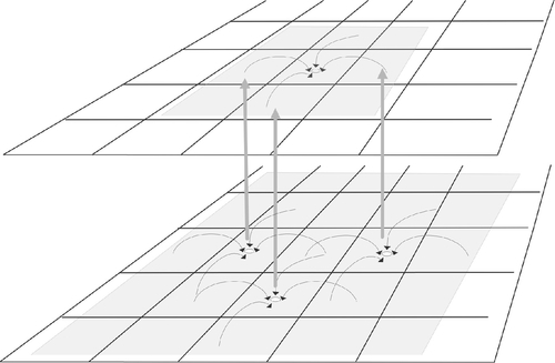
This is certainly the case with multicore processors, where all cores can equally easily read any element from memory. We call this shared memory; see Figure 10.3.

In the CUDA example, each processing element essentially reasoned “this is my number, and therefore I will work on this element of the array” In other words, each processing element assumes that it can work on any data element, and this works because a GPU has a form of shared memory.
While it is convenient to program this way, it is not possible to make arbitrarily large computers with shared memory. The shared memory approaches discussed so far are limited by the amount of memory you can put in a single PC, at the moment about 1 TB (which costs a lot of money!), or the processing power that you can associate with shared memory, at the moment around 48 cores.
If you need more processing power, you need to look at clusters, and “distributed memory programming.”
Distributed memory parallelism
Clusters, also called distributed memory computers, can be thought of as a large number of PCs with network cabling between them. This design can be scaled up to a much larger number of processors than shared memory. In the context of a cluster, each of these PCs is called a node. The network can be Ethernet or something more sophisticated such as Infiniband.
Since all nodes work together, a cluster is in some sense one large computer. Since the nodes are also to an extent independent, this type of parallelism is called multiple instruction, multiple data (MIMD): each node has its own data, and executes its own program. However, most of the time the nodes will all execute the same program, so this model is often called single program, multiple data (SPMD); see Figure 10.4. The advantage of this design is that tying together thousands of processors allows you to run very large problems. For instance, the almost 13,000 processors of the Stampede supercomputer2 (Figure 10.5) have almost 200 TB of memory. Parallel programming on such a machine is a little harder than what we discussed above. First of all we have to worry about how to partition the problem over this distributed memory. But more importantly, our above assumption that each processing element can get hold of every data element no longer holds.

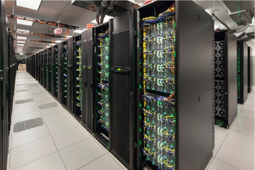
It is clear that each cluster node can access its local problem data without any problem, but this is not true for the “remote” data on other nodes. In the former case the program simply reads the memory location; in the latter case accessing data is possible only because there is a network between the processors: in Figure 10.5 you can see yellow cabling connecting the nodes in each cabinet, and orange cabling overhead that connects the cabinets. Accessing data over the network probably involves an operating system call and accessing the network card, both of which are slow operations.
Distributed memory programming
By far the most popular way for programming distributed memory machines is by using the MPI library. This library adds functionality to an otherwise normal C or Fortran program for exchanging data with other processors. The name derives from the fact that the technical term for exchanging data between distributed memory nodes is message passing.
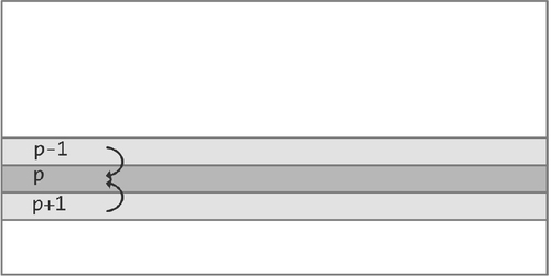
Let us explore how you would do programming with MPI. We start with the case that each processor stores the cells of a single line of the Life board, and that processor p stores line p. In that case, to update that line it needs the lines above and below it, which come from processors p − 1 and p + 1, respectively. In MPI terms, the processor needs to receive a message from each of these processors, containing the state of their line.
Let us build up the basic structure of an MPI program. Throughout this example, keep in mind that we are working in SPMD mode: all processes execute the same program. As illustrated in Figure 10.6, a process needs to get data from its neighbors. The first step is for each process to find out what its number is, so that it can name its neighbors.
Then the process can actually receive data from those neighbors (we ignore complications from the first and the last line of the board here).
With this, it is possible to update the data stored in this process:
(We omit the code for life_line_update, which computes the updated cell values on a single line.) Unfortunately, there is more to MPI than that. The commonest way of using the library is through two-sided communication, where for each receive action there is a corresponding send action: a process cannot just receive data from its neighbors, the neighbors have to send the data.
But now we recall the SPMD nature of the computation: if your neighbors send to you, you are someone else’s neighbor and need to send to them. So the program code will contain both send and receive calls.
The following code is closer to the truth:
Since this is a general tutorial, and not a course in MPI programming, we will leave the example phrased in pseudo-MPI, ignoring many details. However, this code is still not entirely correct conceptually. Let us fix that.
Conceptually, a process would send a message, which disappears somewhere in the network, and goes about its business. The receiving process would at some point issue a receive call, get the data from the network, and do something with it. This idealized behavior is illustrated in the left half of Figure 10.7. Practice is different.

Suppose a process sends a large message, something that takes a great deal of memory. Since the only memory in the system is on the processors, the message has to stay in the memory of one processor, until it is copied to the other. We call this behavior blocking communication: a send call will wait until the receiving processor is indeed doing a receive call. That is, the sending code is blocked until its message is received.
But this is a problem: if every process p starts sending to p − 1, everyone is waiting for someone else to do a receive call, and no one is actually doing a receive call. This sort of situation is called deadlock.
Finding a “clever rearrangement” is usually not the best way to solve deadlock problems. A common solution is to use nonblocking communication calls. Here the send or receive instruction indicates to the system only the buffer with send data, or the buffer in which to receive data. You then need a second call to ensure that the operation is actually completed.
In pseudocode, we have the following:
Task scheduling
All parallel realizations of Life you have seen so far were based on taking a single time step, and applying parallel computing to the updates in that time step. This was based on the fact that the points in the new time step can be computed independently. But the outer iteration has to be done in that order. Right?
Well…
Let us suppose you want to compute the board two time steps from now, without explicitly computing the next time step. Would that be possible?
This exercise makes an important point about dependence and independence. If the value at i,j depends on 3 × 3 previous points, and if each of these have a similar dependence, we can compute the value at i,j if we know 5 × 5 points two steps away, etc. The conclusion is that you do not need to finish a whole time step before you can start the next: for each point update only certain other points are needed, and not the whole board. If multiple processors are updating the board, they do not need to be working on the same time step. This is sometimes called asynchronous computing. It means that processors do not have to synchronize what time step they are working on: within restrictions they can be working on different time steps.
The previous sections were supposed to be about task parallelism, but we did not actually define the concept of a task. Informally, a processor receiving border information and then updating its local data sounds like something that could be called a task. To make it a little more formal, we define a task as some operations done on the same processor, plus a list of other tasks that have to be finished before this task can be finished.
This concept of computing is also known as dataflow: data flows as output of one operation to another; an operation can start executing when all its inputs are available. Another concept connected to this definition of tasks is that of a directed acyclic graph: the dependencies between tasks form a graph, and you cannot have cycles in this graph, otherwise you could never get started….
You can interpret the MPI examples in terms of tasks. The local computation of a task can start when data from the neighboring tasks is available, and a task finds out about that from the messages from those neighbors coming in. However, this view does not add much information.
On the other hand, if you have shared memory, and tasks that do not all take the same amount of running time, the task view can be productive. In this case, we adopt a master-worker model: there is one master process that keeps a list of tasks, and there are a number of worker processors that can execute the tasks. The master executes the following program:
1. The master finds which running tasks have finished.
2. For each scheduled task, if it needs the data of a finished task, mark that the data is available.
3. Find a task that can now execute, find a processor for it, and execute it there.
The pseudocode for this is as follows:
The master-worker model assumes that in general there are more available tasks than processors. In the Game of Life we can easily get this situation if we divide the board into more parts than there are processing elements. (Why would you do that? This mostly makes sense if you think about the memory hierarchy and cache sizes; see Section 1.3 in [2].) So with N × N divisions of the board and T time steps, we define the queue of tasks:
10.3 Advanced topics
10.3.1 Data Partitioning
The previous sections approached parallelization of the Game of Life by taking the sequential implementation and the basic loop structure. For instance, in Section 10.2.3 we assigned a number of lines to each processor. This corresponds to a one-dimensional partitioningof the data. Sometimes, however, it is a good idea to use a two-dimensional one instead. (See Figure 10.8 for an illustration of the basic idea.) In this section you will get the flavor of the argument.

Suppose each processor stores one line of the Life board. As you saw in the previous section, to update that line it needs to receive two lines worth of data, and this takes time. In fact, receiving one item of data from another node is much slower than reading one item from local memory. If we inventory the cost of one time step in the distributed case, that comes down to
1. receiving 2N Life cells from other processors3; and
2. adding 8N values together to get the counts.
For most architectures, the cost of sending and receiving data will far outweigh the computation.
Let us now assume that we have N processors, each storing a ![]() part of the Life board. We sometimes call this the processor’s subdomain. To update this, a processor now needs to receive data from the lines above, under, and to the left and right of its part (we are ignoring the edge of the board here). That means four messages, each of size
part of the Life board. We sometimes call this the processor’s subdomain. To update this, a processor now needs to receive data from the lines above, under, and to the left and right of its part (we are ignoring the edge of the board here). That means four messages, each of size ![]() . On the other hand, the update takes 8N operations. For large enough N, the communication, which is slow, will be outweighed by the computation, which is much faster.
. On the other hand, the update takes 8N operations. For large enough N, the communication, which is slow, will be outweighed by the computation, which is much faster.
Our analysis here was very simple, based on having exactly N processors. In practice you will have fewer processors, and each processor will have a subdomain rather than a single point. However, a more refined analysis gives the same conclusion: a two-dimensional distribution is to be preferred over a one-dimensional one; see, for instance, Section 6.2.2.3 in [2] for the analysis of the matrix-vector product algorithm.
Let us do just a little analysis on the following scenario:
• You have a parallel machine where each processor has an amount M of memory to store the Life board.
• You can buy extra processors for this machine, thereby expanding both the processing power (in operations per second) and the total memory.
• As you buy more processors, you can store a larger Life board: we are assuming that the amount M of memory per processor is kept constant. (This strategy of scaling up the problem as you scale up the computer is called weak scaling. The scenario where you increase only the number of processors, keeping the problem fixed and therefore putting fewer and fewer Life cells on each processor, is called strong scaling.)
Let P be the number of processors, and let N the size of the board. In terms of the amount of memory M, we then have
Let us now consider a one-dimensional distribution (left half of Figure 10.9). Every processor but the first and the last one needs to communicate two whole lines, meaning 2N elements. If you express this in terms of M, you find a formula that contains the variable P. This means that as you buy more processors, and can store a larger problem, the amount of communication becomes a function of the number of processors.

Now consider a two-dimensional distribution (right half of Figure 10.9). Every processor that is not on the edge of the board will communicate with eight other processors. With the four “corner” processors only a single item is exchanged.
The previous two exercises demonstrate an important point: different parallelization strategies can have different overhead and therefore different efficiencies. The one-dimensional distribution and the two-dimensional distribution both lead to a perfect parallelization of the work. On the other hand, with the two-dimension distribution the communication cost is constant, while with the one-dimensional distribution the communication cost goes up with the number of processors, so the algorithm becomes less and less efficient.
10.3.2 Combining Work, Minimizing Communication
In most of the above discussion we considered the parallel update of the Life board as one bulk operation that is executed in sequence: you do all communication for one update step, and then the communication for the next, etc.
Now, the time for a communication between two processes has two components: there is a start-up time (known as “latency”), and then there is a time per item communicated. This is usually rendered as
where the α is the start-up time and β the per-item time.
If the ratio between α and β is large, there is clearly an incentive to combine messages. For the naive parallelization strategies considered above, there is no easy way to do this. However, there is a way to communicate only once every two updates. The communication cost will be larger, but there will be savings in the start-up cost.
First we must observe that to update a single Life cell by one time step we need the eight cells around it. So to update a cell by two time steps we need those eight cells plus the cells around them. This is illustrated in Figure 10.10. If a processor has the responsibility for updating a subsection of the board, it needs the halo regionaround it. For a single update, this is a halo of width 1, and for two updates this is a halo of width 2.
Let us analyze the cost of this scheme. We assume that the board is square of size N × N, and that there are P × P processors, so each processor is computing an (N/P) × (N/P) part of the board.
In the one-step-at-a-time implementation a processor
1. receives four messages of length N and four messages of length 1; and
2. then updates the part of the board it owns to the next time step.
To update its subdomain by two time steps, the following is needed:
1. Receive four messages of size 2N and four messages of size 4.
2. Compute the updated values at time t + 1 of the subdomain plus a locally stored border of thickness 1 around it.
3. Update precisely the owned subdomain to its state at t + 2.
So now you send slightly more data, and you compute a little more, but you save half the latency cost. Since communication latency can be quite high, this scheme can be faster overall.
10.3.3 Load Balancing
The basic motivation of parallel computing is to be able to compute faster. Ideally, having p processors would make your computation p times faster (see Section 2.2 in [2] for a definition and discussion of speedup), but practice does not always live up to that ideal. There are many reasons for this, but one is that the work may not be evenly divided between the processors. If some processors have more work than others, they will still be computing while the others have finished and are sitting idle. This is called load imbalance.
Exercise 12
Compute the speedup from using p processors if one processor has a fraction ![]() more work than the others; the others are assumed to be perfectly balanced. Also compute the speedup from the case where one processor has ϵ less work than all the others. Which of the two scenarios is worse?
more work than the others; the others are assumed to be perfectly balanced. Also compute the speedup from the case where one processor has ϵ less work than all the others. Which of the two scenarios is worse?
Clearly, there is a strong incentive for having a well-balanced load between the processors. How to do this depends on what sort of parallelism you are dealing with.
In Section 10.2.3 you saw that in shared memory it can make sense to divide the work into more units than there are processors. Statistically, this evens out the work balance. On the other hand, in distributed memory (Section 10.2.3) such dynamic assignment is not possible, so you have to be careful in dividing up the work. Unfortunately, sometimes the workload changes during the run of a program, and you want to rebalance it. Doing so can be tricky, since it requires problem data to be moved, and processors have to reallocate and rearrange their data structures. This is a very advanced topic, and not at all simple to do.
10.4 Summary
In this chapter you have seen a number of parallel programming concepts through the example of the Game of Life. Like many scientific problems, you can view this as having parallelism on more than one level, and you can program it accordingly, depending on what sort of computer you have.
• The “data parallel” aspect of the Life board can be addressed with the vector instructions in even laptop processors.
• Just about every processor in existence is also pipelined, and you can express that in your code.
• A GPU can handle fairly fine-grained parallelism, so you would write a “kernel” that expresses the operations for updating a single cell of the board.
• If you have a multicore processor, which has shared memory, you can use a loop-based model such as OpenMP to parallelize the naive code.
• On both a multicore processor and distributed memory clusters you could process the Life board as a set of subboards, each of which is handled by a core or by a cluster node. This takes some rearranging of the reference code; in the distributed memory case you need to insert MPI library calls.
In all, you see that, depending on your available machine, some rearranging of the naive algorithm for Game of Life is needed. Parallelism is not a magic ingredient that you can easily add to existing code, it needs to be an integral part of the design of your program.