
Modules for introducing threads
David P. Bunde* * Knox College
Abstract
This chapter presents a pair of modules for introducing students to parallel programming. Each module is built around an exploratory exercise to parallelize an application, which can be used in a laboratory or a lecture. They illustrate fundamental concepts such as speedup, race conditions, privatizing variables, and load balance. Variations teach students about explicit threading (in C, C++, or Java) and OpenMP (in C/C++).
Relevant core courses: Systems, CS2.
Relevant parallel and distributed computing topics: Shared memory: compiler directives/pragmas (A), libraries (A); Task/thread spawning (A); Data parallel: parallel loops for shared memory (A); Synchronization: critical regions (A); Concurrency defects: data races (C); Load balancing (C); Scheduling and mapping (K); Speedup (C).
Learning outcomes: The student will be able to use common thread libraries for new problems and also have a working knowledge of some basic concepts of parallel programming.
Context for use: First course introducing shared memory programming. Assumes prior background in either Java or C/C++.
4.1 Introduction
This chapter1 presents a pair of modules for teaching basic thread programming. Each module is built around an example application, stepping through the process of parallelizing that application. The first module uses the example of counting the number of primes up to some value. The second uses the example of generating an image of the Mandelbrot set. Each module includes a summary of the author’s experiences teaching it and advice for using it at other institutions.
Target audience
The materials in this chapter are intended for instructors who are introducing their students to parallel programming and concurrency. The author has primarily used these examples in a systems programming course that covers basic operating systems and networking concepts. That course has a CS2 prerequisite, though some students have done additional prior computer science coursework. The modules can also potentially be used late in CS2 or as the first examples in a more advanced course on parallel programming.
Threads and OpenMP
Both modules teach shared memory programming with threads. Such programs use multiple threads to simultaneously execute different parts of the program. Each thread has its own program counter and stack (i.e., distinct local variables), but all the threads run in the same memory space, with interactions through shared variables, either global variables in C/C++ or static variables in Java.
The modules use two different approaches for creating and managing threads. The first is explicit threading, in which the programmer uses system calls to directly create threads and manage interactions between them. The example code does this using the POSIX-standard pthreads library in C, the std::thread class in C++11, and the Thread class in Java. The second thread creation and management approach, used only in the second module, is OpenMP. OpenMP is a standardized extension of C (and C++) in which the compiler generates the thread-related code on the basis of hints (called pragmas) added to a sequential program.
Topics covered
Both modules cover the idea of threads and at least one notation for using them. In addition, they both cover the following concepts:
• Race conditions
• Load balance
• Privatization of variables, the act of giving threads private copies of a variable to reduce the amount of sharing
In addition to these shared concepts, each module covers some additional concepts not included in the other. The prime counting module adds the following:
• Critical sections and mutual exclusion
The Mandelbrot module adds the following:
• Parallel overhead, the extra work added to a program in the process of parallelizing it
• Dynamic scheduling, in which the tasks performed by each thread are determined at run time
Using these modules
The author has typically used only one of these modules in any given course since the modules cover many of the same concepts and class time is always limited. Of the two, the prime counting example seems to be simpler since its given code is shorter and less complicated. Thus, it should be used first if both modules are taught. Language choice may also factor into the decision of which module to use; the prime counting example can be done in Java, C, or C++, while the Mandelbrot exercise must be done in C or C++ since OpenMP is available only in those languages.
Computing environment
The running times discussed in this chapter were measured on two different systems. The majority are from a 16-core AMD Opteron 6272 processor running Fedora Linux release 19. In Section 4.3, we also contrast results on that system with times from a MacBook Pro with a dual-core Intel Core i5 processor (dual-core with hyperthreading support for two tasks per core) running Mac OS X version 10.6.8 (Snow Leopard). The C and C++ examples were compiled using gcc version 4.8.3 on the Linux system and 4.2.1 on the Mac system. On both systems, we used the command line options -Wall (enable all warnings), -lpthread (include the POSIX-standard pthread library to implement threading), -lm (include the math library), and -fopenmp (activate OpenMP; included only when using OpenMP). In addition, the C standard was specified. For C we specified the C 99 standard with -std=c99 (later standards should work as well), and for C++ we specified C++11 with -std=c++11 (required for the C++11 threading). The Java examples were compiled as Java version 1.7. The running times were measured using the Unix command time.
The specific running times will differ depending on your hardware and software configuration, so instructors adopting these materials are encouraged to time the code on their own systems and to rescale the problem sizes.
4.2 Prime counting
This section describes the first module, which is based on a program counting prime numbers. A prime is an integer whose only positive integral divisors are 1 and itself. Primes are one of the main topics of study of number theory, and also have great practical importance in computer cryptography. Their distribution among the integers is related to the Riemann hypothesis, one of the most important open problems in mathematics.
This module was previously presented in [1]; this version expands on that presentation, adding more about the author’s experiences, the C and C++ versions of the module, and a discussion of issues arising with more than two cores. Given code and the author’s handouts for this module are available from [2].
4.2.1 Using this Module
The main part of this module involves walking through the parallelization of a program that counts the number of primes in a range. The author has always done this in a laboratory. The students are given the sequential program and follow the instructions in a handout that lead them through the process of parallelizing it (i.e., the entire process outlined in Section 4.2.3). The instructor is available for questions, but the intent is that the students work through most of the process themselves. Prior to this laboratory, the instructor has briefly introduced the idea of threads in a lecture. Following the laboratory, the instructor also talks about each part of the laboratory to reinforce the lessons learned and to answer questions. Afterward, the students are given a follow-up assignment as homework. (One possible assignment is discussed in Section 4.2.4.)
For courses without class time allocated to working in a laboratory, there are a couple of alternatives. The first is for the parallelization to be done in a lecture, with the instructor illustrating the process. This loses the hands-on aspect since the students are watching rather than changing the code themselves. The second alternative is to give the laboratory handout to students as an assignment. In this case, it would be harder for students to get assistance, but the author does not believe this would be a serious issue since most students in his course completed the laboratory assignment on their own. A potentially bigger concern is that some students may not work on the laboratory assignment, though this would be mitigated by requiring the follow-up assignment.
4.2.2 Sequential Code
Now we describe the initial sequential program that students are given. It has a function isPrime that returns whether its argument is prime. To test the number n for primality, this function tries all integers from 2 to ![]() as possible divisors. (We have to check up only to
as possible divisors. (We have to check up only to ![]() since any divisor above
since any divisor above ![]() will be paired with one below
will be paired with one below ![]() .) The program uses isPrime to count the number of primes up to some value finish, using the code shown in Figure 4.1. This code “prerecords” that 2 is prime and then tests odd integers up to finish.
.) The program uses isPrime to count the number of primes up to some value finish, using the code shown in Figure 4.1. This code “prerecords” that 2 is prime and then tests odd integers up to finish.

For the value of finish, the author used 2,000,000. Adopters of this module should choose a value that is appropriate for the machines with which they are working. The fastest version should take a measurable amount of time, and the sequential version should take at least a couple of seconds. Students are used to instant feedback from their programs and so are strongly motivated to speed this program up so they do not have to wait. (When this example has been used with larger values of finish, some students require reassurance that the initial program is correct because they thought it was in an infinite loop and killed it before completion.)
4.2.3 Step-by-Step Parallelization
Now we step through the process of parallelizing this program. As described above, this is intended as a discovery process, either during a lecture or in a laboratory. Thus, the first versions are incorrect; subsequent versions correct the bugs and then tune the performance.
Creating multiple threads
The first step is creating multiple threads. The main part of this is to move the nextCand loop shown in Figure 4.1 into a function for a thread to run. Each thread will run this function for a different range of candidate numbers. To do this, the thread function needs to know the endpoints of the range of candidate numbers to check. This is simplest in C++,2 where the endpoints can be passed as a pair of integer arguments. These arguments, along with the thread function, are passed to the constructor for std::thread. In C, thread functions take only a single argument, so the endpoints must be placed in a struct. A pointer to this struct is then passed to the pthread_create function, which creates a thread. In Java, threads are represented with Thread objects. The thread body is specified via a Runnable object passed to the constructor, and the range endpoints must be stored as attributes of the Runnable object.
In all three implementations, the threads must be able to increase the count of primes found, which we store in a variable pCount. As a first cut toward updating pCount, we make it a shared variable which each thread increments as primes are found.3 Sketches of the code are shown in Figures 4.2 (C), 4.3 (C++), and 4.4 (Java).


Joining the threads
Running the code in Figure 4.2, 4.3, or 4.4 gives a very underwhelming result. The program is very fast, finishing without noticeable delay, but is incorrect. The C and Java versions find very few primes (possibly none other than 2, which we identified ahead of time). The C++ version exits with an error message: “terminate called without an active exception.” In all cases, the problem is that the program creates and starts the threads, but fails to wait for them to finish before printing the result and exiting. Waiting for thread completion is called joining, a term that captures the idea of the computation that has been distributed over several threads joining together. A single join call waits for a single thread. Thus, we need to add
to the C version of our program,
to the C++ version, or
to the Java version. These calls should be added after both threads have started—that is, after the calls to pthread_create, the declaration of the std::thread objects, or the calls to Thread.start.
Fixing the race condition
After the calls that join the threads have been added, the running time will be more reasonable, but the number of primes found still does not match the (correct) number found by the sequential version. In fact, the number of primes reported by the program likely varies every time the program runs, with the reported number always below the correct value. The variation is caused by a race condition, a concurrency bug in which a bad interleaving of operations executed by different threads can give an incorrect result.
In this case, the problem has to do with the variable pCount, which both threads are updating. Whenever either thread identifies a prime number, it uses the ++ operator to increment this variable. Although the use of a single operator makes this increment appear to be a single operation, executing the operator actually requires three distinct operations: reading the current value of pCount, adding 1 to it, and then storing the new value. If both threads try to increment pCount simultaneously, one of the updates can be lost.
Figure 4.5 depicts one possible way that operations from two threads can interleave and lose an update. It shows the operations of each thread, each thread’s local (register-stored) value of pCount after each operation, and the globally visible value of pCount stored in memory. Initially, pCount has value 5. After both ++ operators have been executed, pCount should have value 7 since it was incremented twice, but instead it has the incorrect value 6; one of the increments has been lost. To make our program properly count the number of primes, we need to avoid this race condition. Specifically, we need one thread to complete the entire ++ operation before the other thread begins it. We can call the line with the ++ operation a critical section, meaning that it is a piece of code that must run all together to guarantee correct execution.

To protect the critical section from interruptions, we will use a lock, also called a mutex because it provides mutual exclusion, the phenomenon of only one thread being in the critical section at a time. Mutexes provide two main operations, lock and unlock. At all times, their state is either locked or unlocked. Mutexes are unlocked when they are created, move to locked if their lock operation is invoked, and move to unlocked if their unlock operation is invoked. Complicating this is that operations that would “change” the state to its current value do not proceed until the state changes. For example, if the lock operation is performed on a mutex that is already locked, that operation will block (i.e., wait) until the mutex becomes unlocked.
A mutex can be used to achieve mutual exclusion for a critical section by adding a call to lock the mutex at the beginning of the critical section and one to unlock it at the end. With this arrangement, any thread wishing to enter the critical section must first lock the mutex, and the mutex remains locked until that thread exits the critical section. Thus, if one thread is in the critical section and another thread attempts to enter it, the second thread will block until the first thread exits the critical section.
To achieve mutual exclusion for our application in C, we replace the single line incrementing pCount with
where m is a global variable for use as a mutex. It is declared and initialized with the following lines:
This ensures that only one thread tries to increment pCount at a time, ensuring that no updates are lost.
The C++ version is similar, albeit with minor syntactic differences since the mutex is now an object. It is declared and initialized with
and then used to protect the increment line with
Note that this code requires including the mutex header file.
There are a couple of differences in how we achieve mutual exclusion in Java. First of all, Java does not have separate lock/mutex objects. Instead, every Java object has an associated mutex. Since the program does not create any objects thus far, we can add one as a class variable:
We could use a different class, but we chose Object to emphasize that the object m is only used as a mutex. Then, to protect the increment operation, we enclose it in a synchronized block:
Despite the difference in syntax, this performs essentially the same operations as the other versions; the mutex associated with m is locked at the beginning of the synchronized block (blocking if necessary), then the increment is performed, and finally the mutex is unlocked. This syntax is less flexible in general, but it makes the relationship between locking and unlocking explicit. It also prevents the programmer from forgetting to unlock a mutex at the end of a critical section.
Now that the code is correct, we can check its performance. On my system, the C version of the sequential code runs in 2.08 s, and the corrected parallel version runs in 1.48 s. (I get slightly different running times for the other versions, but our main focus will be on the ratios between running times, none of which are materially different between the languages.) Thus, it achieves a speedup of 2.08/1.48 = 1.41, meaning that the parallel program runs 1.41 times as fast as the sequential one. This is an improvement, but not very impressive; we would like something closer to linear speedup, a speedup equal to the number of cores we are using. In our case, since we are using two threads and the work they perform is completely independent (since no primality test depends on any other), the goal would be a speedup close to 2.
Privatizing the counter
One possible issue with our parallel program that could be preventing it from achieving a high speedup is the way that it increments pCount. For each increment, the program has to lock and then unlock a mutex. This could undermine our efforts to achieve a high speedup in two ways. First of all, it incurs a relatively high amount of overhead, instructions that are added as part of parallelizing the program. If we execute enough extra instructions, we lose all the benefit of being able to execute instructions faster. Secondly, the mutex causes threads to wait since only one thread can execute the critical section at a time. This is good in that it allows us to achieve mutual exclusion, but having threads wait also undermines the benefit of parallelism. In an extreme case, a program can be completely serialized, meaning that only one thread runs at a time because of mutexes that cause all other threads to block. If this happens, the program gains no benefit from parallelism, while keeping all the additional overhead.
To avoid these issues, we will use a common technique called privatizing variables, in which shared variables are replaced with private copies to eliminate the overhead involved in safely sharing them. In our case, the variable pCount is shared. Looking at this variable, we see the individual threads do not really use its current value. Thus, instead of incrementing pCount each time a prime is found, each thread can have a private counter to record the number of primes it discovers. Then, after the thread has identified all the primes in its range, it can use this private counter to update the shared variable pCount. Since only this last step involves a shared variable, it is the only one that requires protection with a mutex. Figures 4.6 (C), 4.7 (C++), and 4.8 (Java) show the key functions with this modification.


When we run the program after privatizing pCount, we get a minimal improvement in speedup (1.44 from 1.41). For this program, the shared variable was not a big problem. One way to understand this is to observe that the critical section is small relative to the other work each thread is doing, most of which is in the call to isPrime. Since the sequential program spends very little of its time in what becomes the critical section, the threads spend very little time blocked trying to get into it.
Because privatization did not lead to a big performance win in this case, some instructors may want to skip this part of the module. I choose to include it because the technique is important in some cases. In particular, the benefit of privatization increases as the number of threads grows since this makes it more likely that a thread will be in the critical section at any given time. Thus, the technique is likely to become more important over time as processors have more cores.
Improving load balance
Another common factor limiting parallel programming performance, and one that is more important for the prime counting program, is load balance, how evenly the work is divided between the threads. If the work is split unevenly (poor load balance), some threads will take much longer than others. Since the program does not complete execution until the last thread finishes, this makes the overall program slower.
How does this apply to our program? At first glance, the program’s load balance seems good because each thread receives a nearly equal-sized range of numbers to test for primality; the first thread receives 3 through finish/2, while the second receives finish/2 through finish. This impression of equal parts turns out to be an illusion, however, because it takes longer to test the primality of some numbers than others. Consider Figure 4.9, which contains the body of isPrime in Java (the C/C++ version merely replaces Math.sqrt with sqrt and substitutes 0/1 for false/true). This code returns as soon as a divisor of num is found. Thus, its running time is proportional to the value of the smallest divisor for composite (i.e., not prime) numbers and to limit for primes. This leads to the following two opposing arguments about the load balance:

(1) The first thread does more work: There are more prime numbers in the first thread’s range (the lower half), and primes take longer to test than composite numbers.
(2) The second thread does more work: It is testing larger numbers, so its value of limit will be higher. This means its primes require more work than the first thread’s. Composite numbers whose smallest divisor is near the limit will also require more work than composite numbers in the first half.
Empirically, the second argument turns out to be the dominant factor. This can be verified by splitting the numbers unevenly; the program’s running time improves if the ranges are split at a value slightly above finish/2. For example, when finish is 2,000,000, splitting at 1,100,000 improves the speedup to 1.69.
The problem with improving the load balance by adjusting the split point is the difficulty of identifying a good value. For the particular problem of counting prime numbers, there is a clever trick that easily gives good load balance. The idea is to give both threads numbers throughout the entire range; give the first thread numbers of the form 3 + 4k and the second thread numbers of the form 5 + 4k (i.e., start the first thread at 3, start the second thread at 5, and increment by 4 instead of 2 to get the next number). This simple change eliminates the need for tuning the load balance and brings the speedup to 1.86. (One note about this trick: It does not work for odd numbers of threads. For example, applying it with three threads would split the numbers into the forms 3 + 6k, 5 + 6k, and 7 + 6k, but all numbers of the first form are multiples of 3, which are tested very quickly.)
The main part of the module concludes with the corrected load balance, which gives a speedup of 1.86.
4.2.4 Followup Assignment
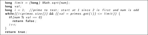
As an exercise related to this module, students were given a homework assignment based on another variation of prime counting. Instead of determining the primality of n by testing all integers from 2 to ![]() , it is sufficient to just test the primes in this range. Figure 4.10 shows the body of a Java function isPrime based on this idea. The variable primes is an ArrayList containing the primes discovered thus far; this list is built as the primes are discovered (by code outside isPrime). Comparison with Figure 4.9 shows that the two methods are quite similar. Avoiding the extra divisor tests yields a large saving, however; the students are given a sequential program utilizing this approach that is actually faster than the best parallelized version based on the previous method.
, it is sufficient to just test the primes in this range. Figure 4.10 shows the body of a Java function isPrime based on this idea. The variable primes is an ArrayList containing the primes discovered thus far; this list is built as the primes are discovered (by code outside isPrime). Comparison with Figure 4.9 shows that the two methods are quite similar. Avoiding the extra divisor tests yields a large saving, however; the students are given a sequential program utilizing this approach that is actually faster than the best parallelized version based on the previous method.
The students’ task was to parallelize this new program, with the suggestion that they sequentially compute the primes up to ![]() . They were also asked in a written question what would go wrong if they just parallelized everything, using the new isPrime with the program developed in the previous section. (The issue is a race condition.) This assignment forces the students to write some threading code outside the laboratory environment. The resulting code is closely related to what they did in the laboratory, but the written question helps check for conceptual understanding.
. They were also asked in a written question what would go wrong if they just parallelized everything, using the new isPrime with the program developed in the previous section. (The issue is a race condition.) This assignment forces the students to write some threading code outside the laboratory environment. The resulting code is closely related to what they did in the laboratory, but the written question helps check for conceptual understanding.
One issue with adapting this assignment for use in C is the lack of a built-in structure equivalent to ArrayList. (Note that it could be replaced with vector in C++.) This issue can be massaged by allocating a sufficiently large array to store the discovered primes, though this approach limits the potential value of final. An alternative is to provide an implementation of an array-based list, but then the students must either trust or understand the given code. (A linked list could also be used, but array-based lists are faster for the operations needed here; the performance is important since the list will be built during the program’s sequential part, before the threads are launched.)
4.3 Mandelbrot
This section describes the second module, which is based on a program creating an image of the Mandelbrot set. The Mandelbrot set is the well-known fractal image depicted in Figure 4.11, where the black points are those inside the set. To determine if a point (x,y) is inside the set, it is interpreted as a complex number c = x + yi, and the series z1 = c, ![]() is computed. Formally, the Mandelbrot set is all points for which this series is bounded. For example, the point (−1,0) is represented as c = z1 = −1, which gives the following series:
is computed. Formally, the Mandelbrot set is all points for which this series is bounded. For example, the point (−1,0) is represented as c = z1 = −1, which gives the following series:
This is clearly bounded, never exceeding magnitude 1. Different behavior is seen for (1,0), which yields a series whose elements’ magnitudes grow without bound:
In practice, depictions of the Mandelbrot set are typically computed by iteratively generating zi until either the magnitude of some zi exceeds a threshold (points outside the set) or a specified number of iterations have been performed (points in the set). The image in Figure 4.11 was generated with a threshold of 2 and by stopping after 1000 elements. For the points above, this would generate all 1000 elements of the series for (−1,0), but would stop the series for (1,0) at z3, the first point whose magnitude exceeds 2.

Users of this module are not required to understand the mathematics behind the Mandelbrot set. The main point is that computing an image such as that shown in Figure 4.11 is a computational task requiring sufficient work to justify parallelization. The only requirement is that the students are able to examine the code determining if a point is in the Mandelbrot set (see Figure 4.13) and observe that its running time varies depending on the iteration at which zi surpasses the threshold.


More information on the Mandelbrot set, including multicolored images that distinguish points on the basis of how soon their series exceeds the threshold, is available from [3]. Given code and the author’s handouts related to this module are available from [4].
4.3.1 Using this Module
As with the prime counting module, the main part of this module is parallelizing a sequential application. Section 4.3.3 steps through the process of doing this using OpenMP, and Section 4.3.4 discusses doing it with explicit threading calls. Since each approach has advantages (discussed in Section 4.3.4), there are many possible ways that this module can be used. Most recently, the author has had students parallelize the program using the approaches one after the other in consecutive laboratory periods (scheduled specifically to facilitate this). Other terms, he has stepped through the OpenMP approach in a lecture either before or after a laboratory in which the students followed the explicit threading approach. His sense is that using a hands-on laboratory was more effective than only lecturing with this material. That said, in courses without a laboratory component, the module could be used as an example for a lecture or students could complete the “laboratory” on their own as an out-of-class activity.
For any of these alternatives, the module should be prefaced by a lecture or reading that briefly introduces the idea of threads. The author also recommends an in-class discussion following the module to reinforce the concepts and answer questions.
The program as given creates an 800 × 800 image of the Mandelbrot set. Depending on the hardware being used, the instructor may wish to adjust this (at the top of the given code) so that the running time is significant but reasonable.
4.3.2 Sequential Program
The initial sequential implementation creates a bitmap file (.bmp). In this type of file, an image is represented as a large array of pixel values. Each pixel is represented by a triple of bytes specifying how much blue, green, and red should appear in a given location. For example, a blue pixel could be represented by setting the blue value as high as possible (255) and setting the other values to 0. Colors other than blue, green, and red are represented as a combination of these three colors. For example, an orange color can be created by setting the red value to 255, the green value to 128, and the blue value to 0. The bulk of the Mandelbrot program’s output is the contents of the array pixels, which stores these color values in structs of type RGBTRIPLE. Each struct has the color of a single pixel, represented by three fields rgbtBlue, rgbtGreen, and rgbtRed that store the values of its blue, green, and red components, respectively. In this program, the only colors we use are black (all values 0) and white (all values 255).
In addition to the array of pixel values, the .bmp file format requires a header. Generating this header requires a significant amount of code, but it does not need to be modified, so it can be treated as a “black box” during parallelization. When the author has used this example in a laboratory, students have been content to ignore this code.
There are only two parts of the program that need to be examined or manipulated. The first part is the pair of loops that we will be parallelizing, shown in Figure 4.12. These loops go through every pixel in the image, whose size is determined by numCols=800 and numRows=800. For each pixel, it calls the function mandelbrot and uses the return value for all three color values for that pixel. Since the calculation for each pixel is independent, these loops are completely parallelizable.
The other part of the program relevant for parallelization is the mandelbrot function, which decides whether a given point (x,y) is in the Mandelbrot set or not. It runs the algorithm described above for 1000 iterations and uses a threshold of 2. (The value appears as 4 in the code because the other side of the inequality is the square of the magnitude.) The function then returns either 0 or 255 depending on whether the given point appears to be in the Mandelbrot set with these parameters—that is, whether ![]() . Code for this method is shown in Figure 4.13.
. Code for this method is shown in Figure 4.13.
4.3.3 Step-by-Step Parallelization with OpenMP
Now we are ready to begin the process of parallelizing this program. As described above, this is intended as a discovery process, either during a lecture or in a laboratory. Thus, our first attempt is incorrect, and subsequent versions fix it and improve the performance.
To make the performance effects as visible as possible, we first set the environment variable OMP_NUM_THREADS to 2, which causes OpenMP to use only two threads. The command to do this varies with the shell being used, but the commands are
for csh or tcsh and
for bash.
Pragma on the outer loop
Since the main work is done in the nested pair of loops shown in Figure 4.12, we focus our parallelization efforts on them. We begin by adding a pragma to run the outer loop in parallel as follows:
After this change, the program does indeed run faster. Unfortunately, it also fails to generate the correct image. Figure 4.14 shows close-ups of the versions generated by the original program and this version. The image generated by the parallel version appears somewhat grainy, with both white pixels inside the set and additional isolated dark ones outside it. (The Mandelbrot set is actually connected, but even the sequential version of our program draws some isolated black pixels since it generates a discrete version of the real set.) In addition, close examination reveals that the parallel version created some pixels with colors other than black and white.

The reason for these artifacts is that both threads created by the pragma are using the same copies of the variables x, y, and color. This causes them to sometimes use a value written by the other thread. Threads interfering with each other in this way is an example of a race condition, a concurrency bug in which a bad interleaving of operations executed by different threads can give an incorrect result.
For example, if the first thread writes 255 in color but the second thread overwrites it with 0 before the first thread sets the pixel values, both threads will store 0 as the pixel values. This causes a pixel that should be white to become black. (The reverse can also happen.) A similar problem can result if the value of x or y is overwritten between when the values are set and when they are used to call the mandelbrot function. Note that these problems occur only when one of the shared variables is changed in the brief time between when it is set and when it is used, which is why most of the pixels have the correct color.
Fixing the race condition
To fix the race condition, we simply want each thread to use its own copies of the variables x, y, and color. To indicate this, we add private(x,y,color) to the end of the pragma, giving the following:
(In this case, the problem could also be solved by declaring these variables within the loop rather than outside it; this is why there are no races on the variable j.) Adding the extra qualifier causes the indicated variables to be privatized—that is, made private to each thread instead of shared by all of them.
After this change, the parallel program produces the same image as the original sequential program. Dividing the sequential running time by the parallel running time gives 1.40. This value, called the speedup, means that the parallel program runs 1.40 times as fast as the sequential version. This is an improvement, but not very impressive. Because every pixel is independent, we would like to achieve something closer to linear speedup, speedup equal to the number of cores in use—that is, two since we limited OpenMP to use two threads.
Swapping the loops
To try improving this, we consider an alternative. What happens if we swap the order of the loops? The resulting code is as follows:
With this change, the speedup becomes 1.94, quite an improvement for such a minor change.
To understand the cause of this change, we have to examine the code of the mandelbrot function in Figure 4.13. Nearly all of this function’s running time is in the while loop. For points in the set (displayed as black in the output and for which the function returns 0), the loop executes 1000 (= maxIteration) times. For points outside the set, the loop exits earlier. Thus, points that are black in the output take longer to process than points that become white.
Now consider how this relates to the change we made by swapping the loops. When the pragma was associated with the i loop, each thread was responsible for a share of the columns. When the loops were reordered, the pragma became associated with the j loop, making each thread responsible for a share of the rows. The two ways of decomposing the image are illustrated in Figure 4.15. As you can see, dividing the rows between threads results in each thread having the same number of black pixels.

Thus, the issue is load balance, how evenly the work is divided between the threads. If the work is split unevenly (poor load balance), some threads take longer than others. Since the program does not complete execution until the last thread finishes, this makes the overall program slower. In our case, splitting the image by rows gives a better load balance than splitting the image by the columns, which explains why parallelizing the j loop gives a better speedup.
The reason for setting the environment variable OMP_NUM_THREADS was to better illustrate this effect. If the variable is not set, OpenMP uses as many threads as can run simultaneously on the hardware. In our case, 16 threads are used, and the resulting speedups are 5.32 when parallelizing the outer loop and 5.98 when parallelizing the inner loop. Swapping the loop order still improves load balance, but less dramatically since the parts are all smaller.
Pragma on the inner loop
A different way to parallelize the j loop is to move the pragma into the outer loop body instead of swapping the loops. This gives the following:
This change gives qualitatively different results depending on the system. The results stated thus far in this chapter are from a 16-core Linux system. On that system, this version of the code gives a speedup of 1.94, the same as the version with swapped loops. On our other system, a dual-core Mac, this version gave a speedup of 1.67, intermediate between the values achieved by the original parallel program (speedup 1.32) and the version with swapped loops (speedup 1.72). (Both systems are described in more detail in Section 4.1.)
Why do the systems give qualitatively different results, and what could cause the intermediate speedup? We begin with the second question and explain the factors that can lead to an intermediate speedup. The version with a parallelized inner loop still has better load balance than the original parallel program; for each column, the work is split between two threads, with each processing the same number of black pixels. There are two reasons why the version with swapped loops may still be better. The first is that it requires fewer instructions. When the inner loop is parallelized, the threads need to start, do their work, and then join each of the numRows times that the outer loop runs. Starting and joining the threads requires extra instructions that do not occur in the sequential version. This extra work is called overhead, instructions that are added as part of parallelizing a program. There is less overhead when the loop order is switched since the threads start and join only once.
A second reason why the swapped version may run faster than the version with a parallelized inner loop has to do with idle time introduced with each join of the threads. When the inner loop is parallelized, there is a join for each column. This means that whichever thread finishes its part of the column first will wait for the other thread before proceeding to the next column. If the threads take different amounts of time for their parts, this difference can accumulate even if the total load is balanced between the threads, as illustrated in Figure 4.16. These differences between thread completion times can occur even if the threads have an identical amount of work because the operating system might not give each of them the same share of the processor. Remember that the operating system is doing other things even if only a single program is running. Random differences in the running time of otherwise identical pieces of work are called jitter.

Given these two factors that tend to favor the version with loops swapped, why does parallelizing the inner loop give the same performance on the Linux system? It turns out that both of these factors are mitigated on that system. To test the overhead, we ran a program that repeatedly created and joined threads with minimal workloads. Overhead caused the parallel version of this program to run more slowly than the serial version on both systems, but the slowdown was less on the Linux system, indicating lower overhead. (The exact cause is unclear, but the Linux system has newer hardware running a more recent operating system and a newer version of the compiler.) The expected effect of jitter is also reduced on the Linux system since it has many cores beyond the two needed for our threads, allowing it to run other things without interrupting our threads.
As a side note, the differences we observed between systems should impress upon readers the need to test the module code on their system before using it in class. With OpenMP, this is particularly important because of the compiler’s increased role. For example, a more aggressive compiler might reorder the nested loops to improve cache performance and thus eliminate the programmer’s ability to try both orders.
Dynamic scheduling
The final step in our illustration of parallelizing the Mandelbrot program is actually an alternative to our manual adjustments to improve load balancing. The idea is to change how the loop iterations are distributed between the threads. Up to this point, all the variations implicitly use what is called static scheduling, meaning that the iterations assigned to each thread are determined before the loop begins. The alternative is dynamic scheduling, in which the iterations are broken into small groups that are then assigned to threads as the loop runs. This requires more coordination between the threads, and the resulting overhead is why static scheduling is the default behavior. For our problem, however, dynamic scheduling improves the load balance by allowing a thread that runs faster iterations to do more of them than a thread that runs slower iterations.
To enable dynamic scheduling, we add schedule(dynamic) to the pragma as follows:
With this change, the program achieves a speedup of 1.94, equal to the bestspeedup previously achieved. The overhead of dynamic scheduling can hurt performance if the iterations are well balanced, but this example shows that it can be very effective when iterations require significantly different amounts of work; dynamic scheduling achieved the same performance without the previous efforts to hand-tune the load balance.
4.3.4 Parallelization Using Explicit Threads
An alternative way to use the Mandelbrot module is to parallelize this program using pthreads, std::thread, or Java threads instead of OpenMP. Hand-written thread code can be used to demonstrate any of the concepts discussed in this section except for dynamic scheduling, which is more complicated to implement by hand. Both the OpenMP approach and the explicit threading approach have advantages. The advantage of OpenMP is that the ease of adding pragmas allows the four main versions of the parallel program (parallelizing i loop or j loop, swapping the loops or not swapping them) to be tested in a relatively short time. Implementing these four versions using explicit threading code would take significantly longer and have a much greater risk that bugs are introduced. Thus, the OpenMP approach is preferable for demonstrating the high-level concepts of load balance and parallel overhead. The disadvantage of using OpenMP instead of explicit threading code is the danger that students see it as “magic” that parallelizes their program without requiring an understanding of the underlying mechanism.
Because of the different advantages of each approach, the author advocates using both when teaching the Mandelbrot module. By the end of the module, the students have both written explicit threading code for a couple of the versions and used OpenMP to explore the entire space of possibilities. The author’s inclination is to take a top-down approach by presenting the idea of threads, having students do the OpenMP version of the module for the high-level concepts, and then having them write explicit threading code. Other instructors could also use this material for a bottom-up approach in which students first write explicit threading code and then move on to OpenMP.