
A Digraph Model for Risk Identification and Management in SCADA Systems
Jian Guan∗, James H. Graham† and Jeffrey L. Hieb†, ∗Department of Computer Information Systems, University of Louisville, Louisville, Kentucky, USA, †Department of Electrical and Computer Engineering, University of Louisville, Louisville, Kentucky, USA
Chapter Outline
4.3 A Digraph Model of SCADA Systems
4.3.1 Structure of SCADA Systems
4.3.2 A Digraph Model of SCADA Systems
4.3.3 Risk Impact and Identification Algorithms
4.1 Introduction
Supervisory control and data acquisition (SCADA) systems are critical to today’s industrial facilities and infrastructures. SCADA systems have evolved into large and complex networks of information systems and are increasingly vulnerable to various types of security risks. SCADA systems play an important role in the daily operation of geographically distributed critical infrastructures such as gas, water and power distribution, and transportation systems such as railways. Early SCADA systems were isolated, proprietary, standalone systems in which cyber or electronic security was largely ignored [1]. However, these systems have undergone tremendous changes in the last few decades and have evolved into complex networks of heterogeneous information systems with highly sophisticated interconnections and interactions [2,3]. The growing dependence of critical infrastructures and industrial automation on these interconnected control systems has resulted in an increasing security threat to SCADA systems [4]. While a major disaster has thus far been averted, there have been incidents such as the 2003 slammer worm penetration of part of a network at a Davis-Besse nuclear power plant in Ohio [5], the release of raw sewage into parks and streams at an Australian sewage treatment plant [6], and the recent hacker penetration of a system used to operate part of a water treatment facility in Harrisburg, PA [7].
Identifying and managing risks in SCADA systems has become critical in ensuring the safety and reliability of these facilities and infrastructure. Most of the existing research on SCADA risk modeling and management has focused on probability-based or quantitative approaches. While probabilistic approaches have proven to be useful, they also suffer from common problems such as simplifying assumptions, large implementation costs, and their inability to completely capture all the important aspects of risk. This chapter presents a digraph model for SCADA systems that allows formal, explicit representation of a SCADA system. A number of risk management methods are presented and discussed for a SCADA system based on the proposed model. In particular, this chapter presents methods for risk impact assessment and fault diagnosis using the proposed model. The approach differs from existing ones in that the proposed methods are mainly based on a model of the structural and functional features of a SCADA system rather than attack and/or vulnerability characteristics, which can be difficult to obtain and are prone to change.
The contributions of the chapter are twofold. First, the proposed model may serve as a conceptual basis for representing both the static and dynamic aspects of a SCADA system for purposes of design, synthesis, and integration. Second, the proposed model can be used for common risk management tasks such as risk assessment and fault diagnosis. The implications for management of SCADA systems are immediate. Managers of SCADA networks need precise and justifiable data about the consequences of specific types of security breaches, and precise and justifiable data about what possible attack consequences are eliminated by specific security measures. The approach proposed here provides managers with both types of data.
The rest of the chapter is organized as follows. The next section provides background and a brief literature review. This is followed by the presentation of the model for SCADA systems. After that two risk management algorithms are proposed for risk assessment and fault diagnosis. Throughout the chapter a SCADA system for a chemical distillation column is used to illustrate the proposed model and algorithms. Finally, in the last section the chapter discusses management implications for the proposed approach to SCADA modeling and risk management.
4.2 Background
SCADA systems have evolved in the last decade into highly complex, interconnected systems. For reasons such as efficiency, cost savings, and integration with enterprise-wide information systems, SCADA systems no longer have dedicated lines of communication. Instead, they share communication channels with the rest of the organization. This change has led to a very different risk profile for SCADA systems and exposed them to the common problems and threats of the Internet [8,9]. This increased level of security threat calls for more rigorous management of SCADA systems to ensure the safe and smooth operations of the underlying infrastructures. Most of the existing research on SCADA security focuses on quantitative/probabilistic risk modeling and analysis. The proposed methods include those based on Hidden Markov Models, statistically based models, and attack trees [4,10–12]. Madan et al. [10] applied a stochastic model to a computer network system to capture attacker behavior and analyze and quantify the security attributes. They determined steady-state availability of quality-of-service requirements and mean times to security failures based on probabilities of failure due to violations of different security attributes. Taylor et al. [12] merged probabilistic risk analysis with survivability system analysis with minor modification of what would be considered traditional probabilistic risk analysis, but it is still dependent on obtaining estimates of probabilities. The ability to determine whether or not risk reduction is achieved when modifications are made is important. Simple calculations for risk reduction have been published [13]. In Tolbert’s paper, a risk metric was calculated that was simply the product of the frequency, likelihood of occurrence, and severity according to an arbitrarily selected scale of 1–5 for each of the three factors. The calculation is made before and after a system modification is made. More recently, McQueen et al. [11] published results of a promising method to calculate risk reduction estimates for a SCADA system and a set of control system remedial actions. The method employed a directed graph (compromise graph) where the nodes represent stages of a potential attack and the edges represent expected time-to-compromise for differing attacker skill levels. Probabilistic risk assessment provides for calculation of risk reduction when applied to SCADA security. If a lower event probability of a specific threat can be set to zero by the addition of a security enhancement, the effect on the top event probability of an overall attack can be computed. Patel et al. [14] have developed a risk modeling tool with two indices for quantifying risk associated with SCADA systems. Their work makes use of augmented vulnerability trees, which combine attack tree and vulnerability tree methods. Attack trees have been applied to a SCADA communication system [4]. The authors identified 11 attacker goals and associated security vulnerabilities in the specifications and development of typical SCADA systems. They were then used to suggest best practices for SCADA operators and improvements to the MODBUS standard. Their application was qualitative in that attack tree analysis was used only to identify paths and qualify the severity of impact, probability of detection, and level of difficulty. They did not calculate the probability of an actual attack being successful.
A common weakness of these methods is their reliability on prior statistical information and/or attack patterns, which are often difficult to obtain. In addition, any solution for SCADA security cannot ignore the importance of the interoperability of these highly complex systems. Igure et al. point out that many proprietary protocols exist in today’s SCADA market [9]. This can make both inter- and intra-company communication difficult, thus adding to the difficulty of risk management for SCADA systems.
4.3 A Digraph Model of SCADA Systems
This section presents a different approach to modeling SCADA systems using a directed graph representation of SCADA systems. First, a general description of SCADA systems is provided and that is followed by the presentation of the proposed digraph model. Finally, a risk impact algorithm and a fault diagnosis algorithm are provided to illustrate how the digraph model can facilitate the risk management task.
4.3.1 Structure of SCADA Systems
A typical SCADA system consists of one or more control centers, one or more field sites, and a communications infrastructure (see Figure 4.1). At the control center a master or master terminal unit (MTU) processes information received from field sites to create a digital representation of the physical process or infrastructure and sends control directives back out to field sites. Operators view the state of the system and issue control directives using various human machine interfaces (HMIs) in the form of operator displays. Field operation is carried out by field devices. Common types of field devices are remote telemetry units (RTUs), intelligent electronic devices (IEDs), and programmable logic controllers (PLCs). The remainder of this chapter will use the term RTU with the understanding that the cyber security-related discussion applies equally well to IEDs and PLCs. RTUs and MTUs are connected by a Wide Area Network (WAN). Possible types of networks include leased lines, Public Switched Telephone Networks (PSTNs), cellular networks, IP-based landlines, radio, microwave and even satellite. A single SCADA system may make use of more than one type of network and the connection between an MTU and RTU may even include more than one type of network technology.

Figure 4.1 Typical SCADA architecture. Adapted from Ref. [15].
4.3.2 A Digraph Model of SCADA Systems
Throughout the discussion in the rest of the chapter, a laboratory-scale distillation column is used as an example of a SCADA system. Figure 4.2 is a schematic diagram of the distillation column SCADA system and Figure 4.3 represents the SCADA system as a digraph.

Figure 4.2 Distillation column schematic.

Figure 4.3 Conceptualization of the distillation column as a digraph.
Let ![]() be a set of components in a SCADA system where xi is a component, such as a master station, submaster station, or an RTU. Then a risk impact relation R can be defined on X such that xiRxj means that components xi and xj are coupled. In others a fault at xi can propagate to xj. A risk impact digraph G is then used to represent this relation as
be a set of components in a SCADA system where xi is a component, such as a master station, submaster station, or an RTU. Then a risk impact relation R can be defined on X such that xiRxj means that components xi and xj are coupled. In others a fault at xi can propagate to xj. A risk impact digraph G is then used to represent this relation as
![]() (4.1)
(4.1)
where
![]() (4.2)
(4.2)
![]() (4.3)
(4.3)
is the edge set. Let A = (aij) be the adjacency matrix representing the risk management digraph such that ![]() and
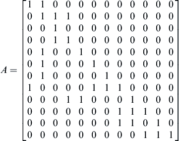
and ![]() . If there is a path in G from xi to xj, xj is said to be reachable from xi. In the context of risk impact assessment or diagnosis this means that a security risk occurring at xi may have a security impact on xj. For completeness every vertex in G is defined to be reachable from itself by a path of 0. As defined above, reachability is transitive. For notational convenience the components in the distillation column example are numbered 1, 2, 3, etc., and the diagraph for the distillation column is as shown in Figure 4.3. The adjacency matrix for the example SCADA system is given as follows:
. If there is a path in G from xi to xj, xj is said to be reachable from xi. In the context of risk impact assessment or diagnosis this means that a security risk occurring at xi may have a security impact on xj. For completeness every vertex in G is defined to be reachable from itself by a path of 0. As defined above, reachability is transitive. For notational convenience the components in the distillation column example are numbered 1, 2, 3, etc., and the diagraph for the distillation column is as shown in Figure 4.3. The adjacency matrix for the example SCADA system is given as follows:
 (4.4)
(4.4)
The reachability matrix P may be defined as follows:
![]() (4.5)
(4.5)
where I is the identity matrix and the operations are Boolean. The reachability matrix P for the digraph in Figure 4.3 is calculated as follows:
 (4.6)
(4.6)
The reachability matrix can be used to derive several important properties describing a SCADA system [16–18]. Two partitions can be defined on the reachability matrix P, the level partition and the separate-parts partition. Let R(x), the reachability set, be the set of vertices reachable from xi and A(xi), the antecedent set, be the set of vertices which reach xi. Then the level partition L(P) is defined as
![]() (4.7)
(4.7)
where k is the number of levels. If the 0th level is defined as the empty set, L0 = ∅, the level partition of P can be found iteratively as follows:
![]() (4.8)
(4.8)
The levels so obtained have the following properties:
• Edges leaving vertices in level Li can go only to vertices in levels Lj such that i ≤ j. In other words, a security risk in components in one level can only impact or propagate to components in the same or lower levels.
Level partitioning can be obtained through tabulation [17]. The level partitions for the distillation column are as follows (shown in Figure 4.4):
![]() (4.9)
(4.9)

Figure 4.4 The level partitions for the distillation column digraph.
It is possible that some of the components of P constitute a smaller digraph that is disjoint from the remainder of the digraph. The separate-parts partition is used to identify these disjoint parts of the SCADA system. To define the separate-parts partition, a set of bottom-level components must be defined. B is a set of bottom-level components, if and only if, for any pi ∈ B:
![]() (4.10)
(4.10)
Given the reachability matrix P for a SCADA system, a separate-parts partition S(P) can be defined as
![]() (4.11)
(4.11)
where m is the number of disjoint digraphs that constitute the digraph represented by A. To find S(P), the set of bottom-level components B must be found, where
![]() (4.12)
(4.12)
Then, any two components xi, xj ∈ B are placed in the same block if and only if:
![]() (4.13)
(4.13)
Once the components of B have been assigned to blocks, the remaining components of the reachability sets for each block are appended to the block.
4.3.3 Risk Impact and Identification Algorithms
One of the main objectives of this chapter is to demonstrate the utility of this SCADA model in managing security risks in a SCADA system. Two such algorithms are presented in this section. The first algorithm allows the assessment of the impact of an at-risk component on a SCADA system. The second algorithm performs fault diagnosis to locate sources of errors.
The first algorithm locates those components that may be affected by a given set of at-risk components. The input to the algorithm are the adjacency matrix A representing the SCADA digraph G and the set of components F that are assumed/known to be at risk. The output of the algorithm is a set of components, O = {x1, x2, x3, …, xn}, that are likely to be affected by the identified security vulnerabilities.
1. Compute the reachability matrix P of G.
2. Compute the level-partition of G.
3. Compute the separate-parts partition of G.
b. Find the leveled impact set ![]() , for i = 1, k, where k is the number of level partitions.
, for i = 1, k, where k is the number of level partitions.
Steps 1–3 preprocess the digraph representing the model by finding the reachability matrix, level partitions, and separate-parts partitions. Step 4a finds the impact set in each separate partition (disjoint digraph). An impact set is defined as the components that may be impacted by the at-risk component(s) in F. It follows that these impact sets represent components in the reachability set(s) of the at-risk components. Step 4b divides each impact set into levels using level partitions. Dividing the impact set components helps distinguish components that are more likely to be impacted from those that are less likely to be impacted. Components in a higher level partition are more likely to be or more immediately affected by the at-risk components because of their closer proximity to the at-risk components. The final output O is the union of all the leveled impact sets in all the partitions.
Again using the distillation column example, assume that the component at risk is F = {11}, then the leveled impact set would be
![]() (4.14)
(4.14)
where
![]() (4.15)
(4.15)
In other words if component 11 is found/assumed to be at risk, then components (1,2,3,4,5,6,7,8,9) are likely to be affected. In addition, from the leveled partition impact sets, it is easy to see that the leveled impact set LQ1 = {(8,9)} is more likely to be immediately affected than the other components. Thus the impact set Q can be used to obtain an assessment of impacted components given a risk alert. Furthermore, the level partitioned impact set, LQ, ranks the set of impacted components in terms of immediacy of impact, so risk reduction methods/action can be directed at those components that are likely to be impacted first.
The model can also be used to support another risk management-related task, i.e. fault diagnosis. Fault diagnosis is a process of locating the components that have led to failure in a SCADA system or parts of a SCADA system. Often when a system fails, the components where failure are observed are not the true causes of failures, but the victims of faults that have propagated from other parts of the system [16,17]. This section presents an algorithm adapted from Ref. [16] for diagnosing faults in a SCADA system given observed symptoms.
Just as in the risk impact assessment algorithm, the diagnostic process starts with the computation of the reachability matrix and the partitions. These are referred to as the preprocessing steps.
DIAGNOSIS
4. T = {x![]() x ∈ Σ and level(x) = min{level(xi) for all xi ∈ Σ}}1
x ∈ Σ and level(x) = min{level(xi) for all xi ∈ Σ}}1
where the TESTCOMPONENTS algorithm is as follows:
TESTCOMPONENTS(T)
4. v ∈ T such that pvz = max{pxz for all x ∈ T and z is the common descendant of all x ∈ T}
7. Test the component v and mark v as tested
8. If the component is abnormal:
10. If the component is tested normal:
11. Remove in A all edges incident to and from v
The above algorithms are designed to assist in the identification of components for testing when a set of components has been observed to have failed/malfunctioned. The objective is to find the source(s) of the failures/malfunctions as it is likely that the observed failures/malfunctions are the result of error propagation originating from components/sources in the higher levels in the digraph. The algorithm starts by finding the common ancestors of the observed failures F and saves the result in Σ (see step 1). This set of common ancestors, Σ, is the set of candidate error sources and is defined as the intersection of the ancestors of the nodes in F (∩ A(xi) for xi ∈ F in step 1). The algorithm will next test the components in Σ and/or their ancestors to identify error sources in steps 3–5. The “while” loop (steps 3–5) examines each of the potential error sources starting with the one at the lowest level of the level-partitioned digraph. Once the component on the lowest level is identified (step 4), a modified depth-first search algorithm (TESTCOMPONENTS) guides the diagnostic process by backtracking along all possible error propagation paths (step 5). In the algorithm TESTCOMPONENTS the input T contains the set of components to examine next. Please note that the first time the algorithm TESTCOMPONENTS is invoked from DIAGNOSIS, T contains only one component. If T contains only one component, this component will be tested (step 7 in TESTCOMPONENTS). Once a component is tested, it is removed from the set of candidate error sources (step 6) and marked as tested (step 7). If the component is normal, the error is unlikely to have originated from its ancestor components further upstream so the related propagation paths are removed from the diagraph, the partitions are recomputed, and the diagnosis process is restarted (restart DIAGNOSIS) (steps 10–13). Otherwise the tested abnormal component is added to the set of error sources Q (step 9). At this point the human operator has the option of stopping the diagnostic process or continuing until all the potential error sources are tested. Steps 14 and 15 will move the search forward by examining the parents of the abnormal node v. If the abnormal node v does not have any parent, the diagnostic process continues with the candidate error source(s) in the next lowest level in the algorithm DIAGNOSIS (step 4 in DIAGNOSIS). If the abnormal node v has parents, they are examined by calling the algorithm TESTCOMPONENTS recursively (step 17 in TESTCOMPONENTS).
There are two possible cases. In the first case there is only a single parent and this parent will be tested (condition in step 1 in TESTCOMPONENTS). In the second case there is more than one parent and the parent from which the error is most likely to have propagated can be determined according to the propagation probabilities. This is to allow the search to stay as closely as possible on the most probable path to the source (step 4). For any component x the error may have propagated from any of the ancestor components upstream. In some cases there may be several immediate ancestors of x and the fault could have propagated from any of these ancestors or any of the error propagation paths headed by these ancestors. Obviously for x a fault may be more likely to propagate from some of the components rather than others. This information can be captured through a propagation probability. Associated with each edge then is pij, the probability that a fault will propagate from xi to xj, 0 < pij ≤ 1. It is assumed that this information is available from users experienced with the SCADA system. In case such information is not available, equal probability can be assigned to each pij and the true probability for pij can be gradually acquired through use of the system [19]. So for each component xj, pij is defined such that ![]() , where n is the in-degree of the vertex representing the component xj. For example, Figure 4.5 shows a component that has three ancestor components that could propagate a fault to it.
, where n is the in-degree of the vertex representing the component xj. For example, Figure 4.5 shows a component that has three ancestor components that could propagate a fault to it.

Figure 4.5 Fault propagation probability.
Step 4 in the TESTCOMPONENTS algorithm directs the search in the most probable path according to the fault propagation probabilities and helps ensure that the search will stay as closely as possible on the most probable path to the fault source. In general, a component is chosen for testing so that the test result can prune away at least one path of components from further consideration.
Thus, the algorithm backtracks along the path until the path branches off into two or more paths. If the component just tested does not have any parent, then the recursive algorithm will allow all other possible error paths to be tested (step 17). Once all possible paths originating from the chosen component in the main algorithm have been examined, the potential error source at the next lowest level will be used to guide the next round of testing (step 4 in the main algorithm). This process continues until all potential error sources in Σ are exhausted.
As an example of a fault diagnosis scenario, assume that a hacker is able to penetrate the corporate network and inject SCADA traffic onto the control network. The hacker may not have any knowledge of the distillation column set up but finds the DNP3 traffic flow on the network. A malicious code injected into the DNP3 (node 11 in Figure 4.4) traffic can result in harm to the distillation column. The injected code/command can tell the devices to directly operate Feed Flow (node 1 in Figure 4.4), Distillation Column (node 2 in Figure 4.4), and/or Reflux Flow (node 5 in Figure 4.4). As a result, for example, the Reflux Flow valve starts to oscillate between 100% open and the target valve steam valve position setting. The other two components may exhibit similar problems. Hence the components F = {1,2,5} may exhibit fault symptoms. The human operator, upon detecting the faulty readings in components 1, 2, and 5, can use the DIAGNOSIS algorithm to locate the source of the faults, i.e. malicious code injected into the DNP3 (node 11 in Figure 4.4). According to the algorithm the only common ancestor to the faulty components is DNP3 (11). As a result {11} will be returned as a probable source of faults. This will alert the operators to take specific and immediate action, such as temporarily raising the security at the control gateway, stopping traffic from the corporate network, etc. See Figure 4.6 for a depiction of the fault scenario. As an example of propagation probabilities guiding the diagnosis process, the distillation column in Figure 4.6 could be part of a larger SCADA system and in a fault diagnosis process component 2 (see Figure 4.4) may have been found to be abnormal. In this scenario the fault could have propagated from one of the four immediate ancestor components {1,5,6,7}. In that case fault propagation probabilities would direct the diagnostic process to search along the most likely path in step 4 of the TESTCOMPONENTS algorithm. This fault diagnosis algorithm can be particularly useful in a large SCADA system that contains hundreds or thousands of components and a timely identification of fault sources is critical.

Figure 4.6 Example fault scenario.
4.4 Conclusions
This chapter presents a digraph model for SCADA systems. A SCADA system, a laboratory-scale distillation column, is used as an example to illustrate the proposed model. The proposed SCADA model offers a simple and easy-to-implement approach for representation of both static and dynamic aspects of a SCADA system. The approach differs from most existing research where the prevalent approach is modeling of risk probabilities or attack patterns. Instead, this model is designed to capture the more fundamental aspects of a SCADA system (i.e. its structure and behavior), and build risk assessment and diagnostic operations from such a model of fundamental aspects. Each component in a SCADA system is represented as a node in a digraph and possible error propagation paths constitute the edges of the digraph. Several important partitions of the digraph can help operators quickly assess impact of possible vulnerabilities and locate error sources. These features of the proposed model are demonstrated through two algorithms. The first algorithm allows an operator to assess the possible impact of security risk in any component or combination of components. The second algorithm assists an operator in locating sources of faults that have been propagated through the system. Such an approach has important advantages. Firstly, the proposed model’s simple structure is easy to implement. In addition to its simplicity most of the information needed for the construction of the model is readily available from system documentation, i.e. structure and function of the system. Secondly, the proposed model may serve as a conceptual basis for representing both the static and dynamic aspects of a SCADA system for purposes of design, synthesis, and integration. Thirdly, the proposed model can be used for common risk management tasks such as risk assessment and fault diagnosis. The implications for management of SCADA systems are immediate. Managers of SCADA networks need precise and justifiable data about the consequences of specific types of security breaches, and precise and justifiable data about what possible attack consequences are eliminated by specific security measures. The approach proposed here provides managers with both types of data.
References
1. McClanahan RH. SCADA and IP: Is network convergence really here?. Ind Appl Mag IEEE. 2003;9(2):29–36.
2. McFarlane DC. Developments in holonic production planning and control. Prod Plan Control. 2000;11(6):522–536.
3. Murray RM, Astrom KJ, Boyd SP, Brockett RW, Stein G. Future directions in control in an information-rich world. IEEE Control Syst Mag. 2003;23(2):20–33.
4. Byres EJ, Franz M, Miller D. The use of attack trees in assessing vulnerabilities in SCADA Systems, International Infrastructure Survivability Workshop (IISW’04). Lisbon, Portugal: IEEE; December 2004.
5. Poulsen K. Slammer worm crashed Ohio nuke plant net. <http://www.securityfocus.com/news/6767> 2003.
6. Smith T. Hacker iailed for revenge sewage attacks. <http://www.theregister.co.uk/2001/10/31/hacker_jailed_for_revenge_sewage/> 2001.
7. Esposito R. Hackers hit Pennsylvania water system. <http://www.isa.org/InTechTemplate.cfm?Section=NewHome&template=/ContentManagement/ContentDisplay.cfm&ContentID=57151> 2006.
8. Brown T. Security in SCADA systems: How to handle the growing menace to process automation. Comput Control Eng. 2005;16(3):42–47.
9. Igure VM, Laughter SA, Williams RD. Security issues in SCADA networks. Comput Secur. 2006;25(7):498–506.
10. Madan BB, Gogeva-Popstojanova K, Vaidyanathan K, Trivedi KS. Modeling and quantification of security attributes of software systems, International Conference on Dependable Systems and Networks. DSN 2002;505–514.
11. McQueen MA, Boyer WF, Flynn MA, Beitel GA. Quantitative Cyber Risk Reduction Estimation Methodology for a Small SCADA Control System. Washington, DC, USA: IEEE Computer Society; 2006.
12. Taylor C, Krings A, Alves-Foss J. Risk analysis and probabilistic survivability assessment (RAPSA): An assessment approach for power substation hardening. Washington, DC: Proc. ACM Workshop on Scientific Aspects of Cyber Terrorism (SACT); 2002.
13. Tolbert GD. Residual risk reduction: systematically deciding what is “safe”. Prof Saf. 2005;50:25–33.
14. Patel SC, Graham JH, Ralston PAS. Security enhancement for SCADA communication protocols using augmented vulnerability trees. Proceedings of the 19th International Conference on Computer Applications in Industry and Engineering 2006;244–251.
15. Stouffer K. NIST industrial control system security activities. Chicago, IL: Proceedings of the ISA Expo; 2005.
16. Guan J, Graham JH. Diagnostic reasoning with fault propagation digraph and sequential testing. IEEE Trans Syst Man Cybern. 1994;24(10):1552–1558.
17. Narayanan NH, Viswanhadam N. A methodology for knowledge acquisition and reasoning in failure analysis. IEEE Trans Syst Man Cybern. 1987;17(2):274–288.
18. Warfield JN. Structuring Complex Systems. Battelle Memorial Institute 1974.
19. Guan J, Graham JH. An integrated approach for fault diagnosis with learning. Comput Indus. 1996;32(1):33–51.
1If there is more than one node at the lowest level in Σ, one of them is chosen randomly to start the testing process.