
APPENDIX E
How to Link Digital Transformation and Value with the Residual Income Valuation Model
The main philosophy behind all conducted financial analysis was to apply a balanced mix of scientific rigor and practitioner‐minded pragmatism for operationalization. This implied no distractions by specialized valuation research models and helped to keep track of accessible digital transformation data, instead of dwelling into theoretical peculiarities of detailed model parametrization. Financial valuation methods have been grouped in many different ways, depending on their objective and approach (Falkum 2011; Vartanian 2003). As indicated earlier, direct and foundational digital transformation, technology/IT/IS, innovation, and corporate finance‐value research over time have applied a seemingly “infinite” variation of customized approaches out of this basket of potential valuation analysis.
From a practitioner perspective, further reviewing this substantial breadth of models was of no further interest for this research, as it has already been extensively analyzed in corresponding meta‐studies, for example, for IT‐payoff (Kohli and Devaraj 2003; Sabherwal and Jeyaraj 2015) or for innovation‐payoff (Vartanian 2003) and, after careful consideration, added no further relevant insights. Instead, the much more promising angle was the subset of approaches, which found theoretically sound ways to integrate nonaccounting “other information” into models otherwise fully based on publicly available financial reporting. After a careful assessment, residual income valuation models, and specifically the Ohlson model (Ohlson 1995, 2001), seemed to be the best starting point. Since being introduced by Ohlson in the 1990s, residual income valuation (RIM) models have opened new possibilities to leverage accounting‐based information in valuation. They have been shown to produce better results than the previously favored cash‐based models (Gao et al. 2019; Ohlson 2001). Nevertheless, in their basic form, they were not without criticism, often with the reproach of systematic undervaluation, as will be elaborated later in more detail.
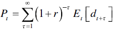
So how does it work? As described by McCrae and Nilsson (2001), whose explanations are used as the basis for summarizing the majority of theoretical foundations in the following, two major assumptions are required for any basic Ohlson‐related model to be valid. First, the market value of a firm's equity ![]() equals the present value of future dividends payments
equals the present value of future dividends payments ![]() . Equity contributions are included as negative dividends. This implies:
. Equity contributions are included as negative dividends. This implies:
In this case ![]() equals the cost of equity capital and
equals the cost of equity capital and ![]() is used as the expectation operator based on available information at time
is used as the expectation operator based on available information at time ![]() .
.
The second assumption calls for the book value changes over time to not oppose the so‐called clean surplus principle. This implies that any change in book value, period to period, is equal to the earnings minus net dividends, resulting in:
Here ![]() equals book value at time
equals book value at time ![]() ,
, ![]() the term for earnings for period
the term for earnings for period ![]() and
and ![]() shows the net dividends given to shareholders at time
shows the net dividends given to shareholders at time ![]() . All valuation‐relevant information needs to be at some point reflected in the profit and loss statements to fulfill the requirements of lean surplus accounting. This establishes the so‐called residual income or abnormal earnings
. All valuation‐relevant information needs to be at some point reflected in the profit and loss statements to fulfill the requirements of lean surplus accounting. This establishes the so‐called residual income or abnormal earnings ![]() :
:
These two equations combine in the valuation function:
Ohlson's major theoretical contribution was an extension to this equation: His “linear information dynamics” (LIM) solved the limitation that it is only based on future values and thus does not allow to link publicly available accounting figures to equity value. For Ohlson, the information of expected future abnormal earnings was based on both the history of abnormal earnings and non‐accounting “other information” not reflected in this history ![]() . He then postulated a modified first‐order autoregressive process for these abnormal earnings and a simple first‐order autoregressive process for non‐accounting information.
. He then postulated a modified first‐order autoregressive process for these abnormal earnings and a simple first‐order autoregressive process for non‐accounting information.
This gives for abnormal earnings (or residual income):
For non‐accounting “other information,” this implies:
Here ![]() and
and ![]() are fixed persistence parameters that are supposed to be transparent, greater than zero, and less than one. The variable
are fixed persistence parameters that are supposed to be transparent, greater than zero, and less than one. The variable ![]() represents non‐accounting information on expected future abnormal earnings that is seen at the end of period
represents non‐accounting information on expected future abnormal earnings that is seen at the end of period ![]() but not yet reflected in accounting, and
but not yet reflected in accounting, and ![]() represents a random error term assumed to be mean zero and uncorrelated over time.
represents a random error term assumed to be mean zero and uncorrelated over time.
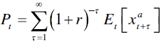
Ohlson's other important contribution was to fix the finite valuation problem embedded in most traditional models: Assuming a ![]() and
and ![]() of below one, abnormal earnings converge to zero, so that in the long run the firm's book and market value will converge. This fits to the theoretical notion that efficient market competition should eventually cancel out firm‐specific abnormal earnings. This leads to a valuation function for market value based on abnormal earnings, accounting book values and non‐accounting information:
of below one, abnormal earnings converge to zero, so that in the long run the firm's book and market value will converge. This fits to the theoretical notion that efficient market competition should eventually cancel out firm‐specific abnormal earnings. This leads to a valuation function for market value based on abnormal earnings, accounting book values and non‐accounting information:
where:
This new theoretical approach finally laid a foundation for applying accounting data to explain and predict market values, where shareholder value consequently has three major elements: the current book value, the capitalized current residual income, and the capitalized value implied by nonaccounting “other information.” Investors are, in other words, presumed to trade current asset value for a future stream of expected income. Correspondingly, asset prices embody the present value of all future dividends expected. The Ohlson model “… replaces the expected value of future dividends with the book value of equity and current earnings … based on the already explained clean surplus principle, which holds that the change in book value of equity will be equal to earnings less paid out dividends and other changes in capital contributions” (Muhanna and Stoel 2010, p. 50).
In operational implementation terms, this leads to the following regression:
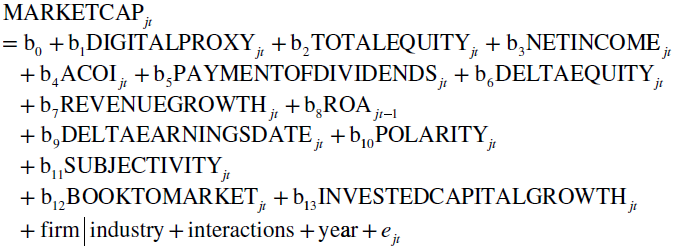
where ![]() is the fiscal year‐end equity market value for firm
is the fiscal year‐end equity market value for firm ![]() for year
for year ![]() ,
, ![]() is our proxy variable,
is our proxy variable, ![]() is the fiscal year‐end book value of equity,
is the fiscal year‐end book value of equity, ![]() is net income,
is net income, ![]() is accumulated other comprehensive income, and
is accumulated other comprehensive income, and ![]() and
and ![]() are dividends paid minus changes in contributed capital, derived from sales of common and preferred stock minus purchases of common and preferred stock. All other parameters are self‐explanatory financial key performance indicators (KPIs) or sentiment parameters as controls except for
are dividends paid minus changes in contributed capital, derived from sales of common and preferred stock minus purchases of common and preferred stock. All other parameters are self‐explanatory financial key performance indicators (KPIs) or sentiment parameters as controls except for ![]() which describes the difference in days between the earnings call and the following submission of information to the SEC. Differences in market values beyond book value and earnings are reflected in
which describes the difference in days between the earnings call and the following submission of information to the SEC. Differences in market values beyond book value and earnings are reflected in ![]() and
and ![]() is the error term. Year and firm|industry indicate the found time and firm/industry fixed effects, interactions the possible variable interactions.
is the error term. Year and firm|industry indicate the found time and firm/industry fixed effects, interactions the possible variable interactions.
The clean surplus rule, as just elaborated, is one key assumption underlying the applicability of the Ohlson model. Even though US‐GAAP, the applicable accounting standards used for all financial information sources in this research, are seen as superior to European accounting standards in this regard, they still include several violations (Falkum 2011; Lo and Lys 2000). Fortunately, FASB Statement No. 130, “Reporting Comprehensive Income,” partially mitigates this, as it requires transparency of all income‐neutral but equity‐influencing actions in the financial statement, so that overall the assumption of clean surplus validity seemed to be fair to make (Falkum 2011) also for the sake of this research, when including this information.
Due to its wide application and acceptance, residual income models (RIM) like the chosen Ohlson model (OM) enjoy the benefit of having been very broadly tested empirically over the past years (Callen and Segal 2005) as summarized in Table E.1. While “accounting based valuation models studies of US firms tend to support Ohlson's proposition that residual and book value numbers have information content in explaining observed market values” (McCrae and Nilsson 2001, p. 315), potential weaknesses are also very transparent. This enables a much more educated discussion of empirical results compared to other, more custom models.
TABLE E.1 Residual income model research overview.
| Author | Research Focus | Results |
|---|---|---|
| Barth et al. (1999) | Implementation and empirical tests of different variants Analysis of industry impact | Better results with decomposed income models Industry‐specific parameters provide better results |
| Biddle, Chen, and Zhang (2001) | Expansion of OM Empirical tests of different hypothesis | Investments correlate with investment return Convexity of current and future residual incomes |
| Choi, O'Hanlon, and Pope (2003) | Expansion of OM by newly developed conservatism | Approach improves OM model |
| Dechow, Hutton, and Sloan (1999) | Implementation of Ohlson model (OM) supplemented by analyst forecasts Using different persistence parameters | Tendency of undervaluation Analyst forecasts have strong influence on investors expectation building |
| McCrae and Nilsson (2001) | Country specifics | Significant differences in results between US and non‐US firms (Sweden) |
| Myers (2000) | Implementation of OM without other information and variations | All methods tend to undervalue Tendency to project too low residual earnings |
| Ota (2002) | Empirical tests of different variants | Tendency of undervaluation Analyst forecasts help to explain market values and investor expectation building |
Implications for this book are manifold. Primarily, the repeating theme of undervaluation leads to the necessity of carefully interpreting results. Furthermore, the value of adding analyst forecasts seems to be visible. Nevertheless, the author has, for the sake of easier operationalization, decided to stick to a simpler version of the Ohlson model, noting the inclusion of analyst expectations as a further potential improvement for later research. Industry relevance has been taken care of insofar as all “other information” variables applied in this research (digital transformation textual analysis‐based variables) are mostly industry‐, or even company‐specific, including the application of firm and industry fixed effects.
TABLE E.2 Model operationalization overview.
| Author | Underlying Research Field | Model Option Description | Evaluation |
|---|---|---|---|
| Anderson, Banker, and Ravindran (2006) | IT value | Custom model | Theoretical foundation available Less relevant as focused only on Y2K event |
| Beutel (2018) | Digital transformation value | Custom model | Theoretical foundation available All required variables available in chosen data sources but different focus |
| Chen and Srinivasan (2019) | Digital transformation value | Custom model | Theoretical foundation available Medium feasibility of operationalization due to high complexity |
| Hossnofsky and Junge (2019) | Digital transformation value | Custom model | Theoretical foundation available High feasibility of operationalization but different focus (analyst view) |
| Mani, Nandkumar, and Bharadwaj (2018) | Digital transformation value | Custom model | Theoretical foundation available High feasibility of operationalization but different focus |
| Mithas, Ramasubbu, and Sambamurthy (2011) | IT value | Custom model | Theoretical foundation available Only questionnaire based |
| Muhanna and Stoel (2010) | IT value | Basic Ohlson model | Strong theoretical foundation All required variables available in chosen data sources |
| Vartanian (2003) | Innovation value | Custom model | Strong theoretical foundation Innovation‐centric variables |
Muhanna and Stoehl's basic Ohlson model operationalization (Muhanna and Stoel 2010) served as a foundation for this research after intense consideration mainly for four reasons. First, it is based on a valid theoretical background as demonstrated. Second, its strong requirement for the clean surplus rule, which otherwise is not easy to meet for all international accounting standards, here can as already discussed be assumed to match with “United States Generally Accepted Accounting Principles” applicable (US GAAP) for the selected companies. Third, the transparency on its weaknesses, based on previous authors' extensive empirical testing, allowed having a better sense for the interpretation of results. Fourth, a final, careful evaluation of potential alternative models, from foundational IT value and innovation value research, identified no better match in terms of theoretical foundation and feasible, thesis‐objective‐supporting operationalization of variables.
While the market value impact of digital transformation is by design of major interest for this research, it seemed advisable to look at least into one more directly accounting‐driven parameter as well. Future earnings were the most obvious choice, given their relevance also in the market value considerations. Instead of developing our own customized model for future earnings analysis, it seemed best to again follow Muhanna and Stoel (2010) and their approach. Other than for the Ohlson model, no extensive empirical tests for the chosen mixed fundamental model exist. Therefore, potential shortcomings have to be fully addressed with our own statistical robustness tests when discussing empirical results. Because no logical or empirical results dictated otherwise, the same approach as selected for residual income regressions was also applied for the mixed fundamental model. To later test the hypothesis on the link of digital transformation with lagged (future) earnings, the herewith applied earnings prediction model fully followed the ideas of Muhanna and Stoel (2010). It combines elements of other earnings prediction approaches used in the literature. The custom final model for future earnings accounted for firm assets plus the historical earnings for the assets. It used the average of return on assets ![]() over three years as the measure of future earnings to allow for a possible lag between digital transformation parameters and the realization of potential value.
over three years as the measure of future earnings to allow for a possible lag between digital transformation parameters and the realization of potential value.
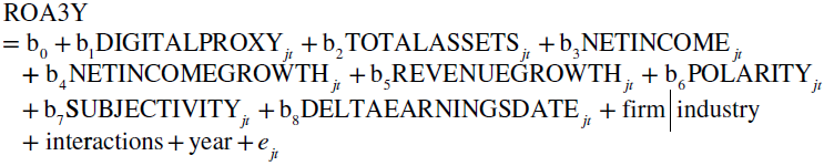
where all variables are self‐explanatory for firm ![]() in year
in year ![]() and year and firm|industry indicate the found time and firm/industry fixed effects, interactions the possible variable interactions, and
and year and firm|industry indicate the found time and firm/industry fixed effects, interactions the possible variable interactions, and ![]() is the error term.
is the error term.
In summary, financial analysis produced several variables, sourced mostly via Intrinio APIs with by design self‐explanatory abbreviations in line with the equations explained earlier. To ensure normality of the dependent variables, both applied variables (MARKETCAP and ROA3Y) were checked for normality, and afterwards natural logged in the final models to account for the identified non‐normality. Other transformation methods like the two‐step or winsorizing approaches as proposed in related literature (Templeton and Burney 2017) were disregarded due to the fact that already simple natural log normalization provided satisfactory results.