
Chapter 26
Model Voting and Propensity Averaging
In Part 6: Enhancing Model Performance, we are examining methods for improving the performance of our classification and prediction models. In Chapter 24, we learned about segmentation models, where useful segments of the data are leveraged to enhance the overall effectiveness of the model. Then, in Chapter 25, we learned about ensemble methods, which combine the results from a set of classification models, in order to increase the accuracy and reduce the variability of the classification. Now, here in this chapter, we consider methods for combining different types of models, using model voting and propensity averaging.
26.1 Simple Model Voting
In Olympic figure skating, the champion skater is not decided by a single judge alone, but by a panel of judges. The preferences of the individual judges are aggregated using some combination function, which then decides the winner. In data analysis, different classification models (e.g., CART (classification and regression trees) vs logistic regression) may provide different classifications for the same data. Thus, data analysts may also be interested in combining classification models, using model voting or propensity averaging, so that the strengths and weaknesses of each model are smoothed out through combination with the other models. Model voting and propensity averaging are considered to be ensemble methods, because the ultimate classification decision is based, in part, on the input from each of the base classifiers.
One method of combining models is to use simple voting (also called majority classification). Consider Table 26.1. Suppose we have a classification task, with a flag target. We develop three independent classification models: (i) a CART model, (ii) a logistic regression model, and (iii) a neural network model. For each record, each model supplies a classification of either response (1) or non-response (0). Table 26.1 shows five records, with the classification supplied by each model, along with the “winning” classification, as tabulated by majority vote among the three classification models.
Table 26.1 Example of simple model voting
| Records | CART | Logistic Regression | Neural Network | C5.0 | Naïve Bayes | Majority Classification |
| 1 | 0 | 0 | 0 | 0 | 0 | 0 |
| 2 | 0 | 1 | 0 | 0 | 0 | 0 |
| 3 | 0 | 1 | 0 | 0 | 1 | 0 |
| 4 | 1 | 1 | 0 | 0 | 1 | 1 |
| 5 | 1 | 1 | 1 | 1 | 1 | 1 |
In this case, the logistic regression model was more likely to classify the records as 1, while the neural network model was less likely. The simple voting scheme is a way of averaging out these predictions, in the hopes that such a consensus model will provide more stable results. This process is analogous to bootstrap aggregation (bagging). However, in bagging, the classification models are the same while the records are resampled. Here, with simple model voting, the models may be different, as in Table 26.1.
26.2 Alternative Voting Methods
Note that the majority classification is only one way of counting the votes of the models. Here follows a list of possible ways of combining the votes of binary classification models:
- Majority Classification. The classification with more than 50% of the votes is selected.
- Plurality Classification. The classification with more votes than any other classification is selected, without having to achieve a majority. For binary classification models, majority classification and plurality classification are equivalent.
- Single Sufficient Classification. If at least one model votes positive, then the combination classification is positive.
- Twofold Sufficient Classification. If at least two models vote positive, then the combination classification is positive.
- k-Fold Sufficient Classification. If at least k models vote positive, then the combination classification is positive, where k < m (total number of models).
- Positive Unanimity Classification. The combination classification is positive only if all models vote positive.
(Of course, there are analogous methods for counting the negative votes.) Note that these alternative methods of counting votes often result in different classification decisions for the combination classifier. Table 26.2 shows the classification decisions made for each different method of counting the votes, for the data from Table 26.1.
Table 26.2 Alternative voting methods lead to different winners
| Records | Plurality Classification | Single Sufficient | Twofold Sufficient | Threefold Sufficient | Fourfold Sufficient | Positive Unanimity |
| 1 | 0 | 0 | 0 | 0 | 0 | 0 |
| 2 | 0 | 1 | 0 | 0 | 0 | 0 |
| 3 | 0 | 1 | 1 | 0 | 0 | 0 |
| 4 | 1 | 1 | 1 | 1 | 0 | 0 |
| 5 | 1 | 1 | 1 | 1 | 1 | 1 |
What are the characteristics of the ensemble models associated with these different voting methods?
- Single sufficient classification is highly aggressive in recognizing positive responses. Thus, its sensitivity1 may be high, but it may also be prone to making a higher number of false positive predictions.
- By contrast, positive unanimity classification is resistant to recognizing positive responses. Hence, while its specificity2 may be high, it may nevertheless be in danger of having too many false negatives.
- We would expect that majority classification would fall somewhere between the behaviors in the previous two bullets, having moderate rates of all four statistics cited. Also, for combining m models (where m is odd), we would expect
 classification to reflect the behavior of the majority classification strategy.
The downside of ensemble classifiers in general extends to voting models; that is, their lack of interpretability. It may be more difficult to explain to a client how a voting ensemble works, compared to the straightforward interpretability of decision trees.
26.3 Model Voting Process
The model voting process is illustrated in Figure 26.1, and may be summarized as follows:
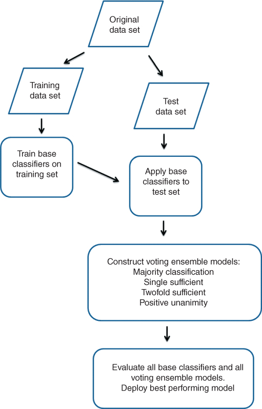
Figure 26.1 Model voting process.
26.4 An Application of Model Voting
To illustrate the application of simple model voting and alternative voting methods to actual data, the model voting process was applied to the ClassifyRisk data set.
- The data set was partitioned into a training data set and a test data set.
- The following base classifiers were trained to predict Risk, using the training set:
- Bayesian network
- Logistic regression
- Neural network.
- For the purposes of this example, a random sample of 25 records was taken from the test data set, to be referred to as the working test data set. Each of the three base classifiers from step 2 was applied to the working test data set.
- The classification results from the three base classifiers were combined into voting ensemble models, using the following voting methods:
- Majority classification
- Single sufficient classification
- Twofold sufficient classification
- Positive unanimity classification.
- Each of the base classifiers from step 3 and each of the four voting ensemble models from step 4 were evaluated with respect to overall error rate, sensitivity, specificity, PFP, and PFN.
The working test data set is shown in Table 26.3, along with the classification results from the three base classifiers in step 2 and the four voting ensemble models in step 5. Risk represents the actual outcome, and the columns to the right of Risk represent the predictions of the base classifiers and the voting ensemble models. (Good Risk is coded as 1, Bad Loss is coded as 0, and Income is rounded to the nearest dollar to save space.) Tables 26.4–26.10 represent the contingency tables of each base classifier and voting model.
Table 26.3 Working test data set
| Mort | Loans | Age | Marital Status | Income | Risk | Bayes Net | Log Reg | Neural Net | Majority | Single Sufficient | Twofold Sufficient | Positive Unanimity |
| Y | 2 | 33 | Other | 31,287 | 0 | 0 | 0 | 0 | 0 | 0 | 0 | 0 |
| Y | 2 | 39 | Other | 30,954 | 0 | 0 | 0 | 0 | 0 | 0 | 0 | 0 |
| Y | 1 | 17 | Single | 27,948 | 0 | 0 | 0 | 0 | 0 | 0 | 0 | 0 |
| Y | 2 | 43 | Single | 37,036 | 0 | 0 | 0 | 0 | 0 | 0 | 0 | 0 |
| Y | 2 | 34 | Single | 23,905 | 0 | 0 | 0 | 0 | 0 | 0 | 0 | 0 |
| Y | 1 | 28 | Married | 38,407 | 0 | 1 | 1 | 0 | 1 | 1 | 1 | 0 |
| N | 1 | 23 | Married | 23,333 | 0 | 0 | 0 | 0 | 0 | 0 | 0 | 0 |
| N | 2 | 38 | Other | 32,961 | 0 | 0 | 0 | 0 | 0 | 0 | 0 | 0 |
| Y | 2 | 26 | Other | 28,297 | 0 | 0 | 0 | 0 | 0 | 0 | 0 | 0 |
| Y | 2 | 43 | Other | 28,165 | 0 | 0 | 0 | 0 | 0 | 0 | 0 | 0 |
| N | 2 | 46 | Other | 27,869 | 0 | 0 | 0 | 0 | 0 | 0 | 0 | 0 |
| Y | 2 | 33 | Other | 27,615 | 0 | 0 | 0 | 0 | 0 | 0 | 0 | 0 |
| Y | 3 | 41 | Other | 24,308 | 0 | 0 | 0 | 0 | 0 | 0 | 0 | 0 |
| Y | 1 | 53 | Single | 35,816 | 0 | 1 | 0 | 1 | 1 | 1 | 1 | 0 |
| Y | 2 | 42 | Single | 24,534 | 0 | 0 | 0 | 0 | 0 | 0 | 0 | 0 |
| Y | 1 | 62 | Single | 33,139 | 1 | 1 | 1 | 1 | 1 | 1 | 1 | 1 |
| N | 1 | 25 | Single | 34,134 | 1 | 0 | 0 | 0 | 0 | 0 | 0 | 0 |
| Y | 2 | 49 | Single | 31,363 | 1 | 1 | 0 | 0 | 0 | 1 | 0 | 0 |
| N | 1 | 35 | Single | 28,277 | 1 | 0 | 0 | 0 | 0 | 1 | 0 | 0 |
| N | 1 | 30 | Married | 49,751 | 1 | 1 | 1 | 1 | 1 | 1 | 1 | 1 |
| N | 1 | 56 | Married | 47,412 | 1 | 1 | 1 | 1 | 1 | 1 | 1 | 1 |
| Y | 1 | 47 | Married | 47,665 | 1 | 1 | 1 | 1 | 1 | 1 | 1 | 1 |
| N | 1 | 48 | Married | 41,335 | 1 | 1 | 1 | 1 | 1 | 1 | 1 | 1 |
| N | 0 | 43 | Single | 55,251 | 1 | 1 | 1 | 1 | 1 | 1 | 1 | 1 |
| Y | 1 | 48 | Single | 40,631 | 1 | 1 | 1 | 1 | 1 | 1 | 1 | 1 |
Table 26.4 Bayesian networks model
| Predicted Risk | |||
| 0 | 1 | ||
| Actual Risk | 0 | 13 | 2 |
| 1 | 2 | 8 | |
Table 26.5 Logistic regression model
| Predicted Risk | |||
| 0 | 1 | ||
| Actual Risk | 0 | 14 | 1 |
| 1 | 3 | 7 | |
Table 26.6 Neural networks model
| Predicted Risk | |||
| 0 | 1 | ||
| Actual Risk | 0 | 14 | 1 |
| 1 | 3 | 7 | |
Table 26.7 Majority voting ensemble model
| Predicted Risk | |||
| 0 | 1 | ||
| Actual Risk | 0 | 13 | 2 |
| 1 | 3 | 7 | |
Table 26.8 Single sufficient ensemble model
| Predicted Risk | |||
| 0 | 1 | ||
| Actual Risk | 0 | 13 | 2 |
| 1 | 2 | 8 | |
Table 26.9 Twofold sufficient ensemble model
| Predicted Risk | |||
| 0 | 1 | ||
| Actual Risk | 0 | 13 | 2 |
| 1 | 3 | 7 | |
Table 26.10 Positive unanimity ensemble model
| Predicted Risk | |||
| 0 | 1 | ||
| Actual Risk | 0 | 15 | 0 |
| 1 | 3 | 7 | |
Table 26.11 contains the model evaluation measures for all of the models. Each of the base classifiers share the same overall error rate, 0.16. However, the positive unanimity ensemble model has a lower overall error rate of 0.12. (The best performance for each of the models is shown in bold.) As expected, the single sufficient model has the best sensitivity and PFN among the ensemble models, but does not perform so well with respect to specificity and PFP. The positive unanimity model does very well in specificity and PFP, and not so well in sensitivity and PFN.
Table 26.11 Model evaluation measures for all base classifiers and voting ensembles (best performance in bold).
| Model | Overall Error Rate | Sensitivity | Specificity | PFP | PFN |
| Bayesian networks | 0.16 | 0.80 | 0.87 | 0.20 | 0.13 |
| Logistic regression | 0.16 | 0.70 | 0.93 | 0.12 | 0.18 |
| Neural networks | 0.16 | 0.70 | 0.93 | 0.12 | 0.18 |
| Majority vote | 0.20 | 0.70 | 0.87 | 0.22 | 0.19 |
| Single sufficient | 0.16 | 0.80 | 0.87 | 0.20 | 0.13 |
| Twofold sufficient | 0.20 | 0.70 | 0.87 | 0.22 | 0.19 |
| Positive unanimity | 0.12 | 0.70 | 1.00 | 0.00 | 0.17 |
This example demonstrates that a well-chosen voting ensemble scheme can sometimes lead to better performance than any of the base classifiers. In effect, voting enables an ensemble classifier to be better than the sum of its parts. Of course, such an improvement in performance is not guaranteed across all data sets. But it is often worth a try.
26.5 What is Propensity Averaging?
Voting is not the only method for combining model results. The voting method represents, for each model, an up-or-down, black-and-white decision without regard for measuring the confidence in the decision. The analyst may prefer a method that takes into account the confidence, or propensity, that the models have for a particular classification. This would allow for finer tuning of the decision space.
Fortunately, such propensity measures are available in IBM/SPSS Modeler. For each model's results, Modeler reports not only the decision, but also the confidence of the algorithm in its decision. The reported confidence measure relates to the reported classification. Because we would like to do calculations with this measure, we must first transform the reported confidence into a propensity for a particular class, usually the positive class. For the ClassifyRisk data set, we do this as follows:

For an ensemble of m base classifiers, then the mean propensity, or average propensity, is calculated as follows:
We may then combine several classification models of various types, such as decision trees, neural networks, and Bayesian networks, and find the mean propensity for a positive response across all these models.
Note that the mean propensity is a field that takes a value for each record. Thus, we may examine the distribution of mean propensities over all records, and select a particular value that may be useful for partitioning the data set into those for whom we will predict a positive response, and those for whom we will predict a negative response.
26.6 Propensity Averaging Process
The propensity averaging process is illustrated in Figure 26.3, and may be summarized as follows:

Figure 26.2 Distribution of mean propensity, with Income overlay.
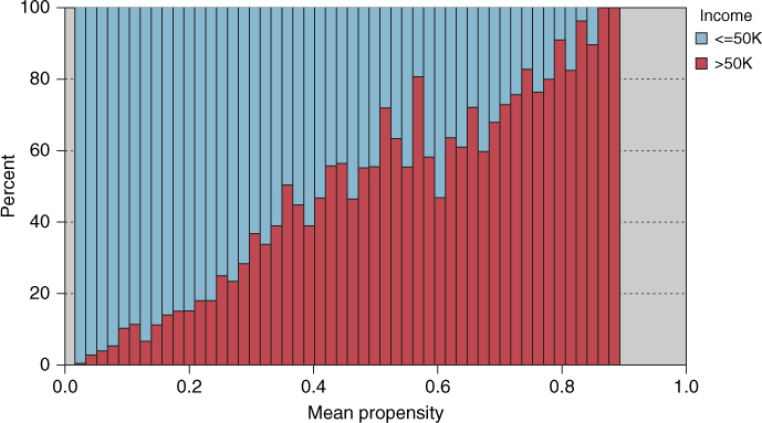
Figure 26.3 Propensity averaging process.
26.7 An Application of Propensity Averaging
The construction of a propensity-averaged ensemble classification model is illustrated using the Adult2_training data set and the Adult2_test data set. The binary target variable Income indicates whether income is above $50,000 or not. The propensity averaging process was applied, and is as follows:
- The Adult data set was partitioned into a training data set and a test data set.
- The following base classifiers were trained to predict Risk, using the training set:
- CART
- Logistic regression
- Neural network.
- Each of the three base classifiers from step 2 was applied to the test data set.
- For each record in the test data set, the propensity of that record toward a positive response (Income > $50,000) was calculated, for each of the base classifiers. The mean propensity was then computed for each record.
- A normalized histogram of the mean propensity, with an overlay of Income, was constructed (Figure 26.2).
Table 26.12 Candidate mean propensity threshold values, with evaluative measures (best performance in bold).
Threshold Value Overall Error Rate Sensitivity Specificity PFP PFN 0.34 0.1672 0.7346 0.8639 0.3689 0.0887 0.4 0.1610 0.6158 0.9097 0.3163 0.1180 0.6 0.1691 0.4477 0.9523 0.2517 0.1552 0.4005 0.1608 0.6158 0.9099 0.3158 0.1180 0.4007 0.1607 0.6158 0.9101 0.3153 0.1180 0.4009 0.1608 0.6151 0.9101 0.3156 0.1182 CART 0.1608 0.5436 0.9328 0.2806 0.1342 Log Reg 0.1748 0.5105 0.9249 0.3171 0.1436 Neur Net 0.1688 0.5388 0.9238 0.3085 0.1366 - The histogram in Figure 26.2 was then scanned from left to right, to identify candidate threshold values of the mean propensity for partitioning the test set into those with positive and negative values for the target, Income. The goal is to select a set of candidate threshold values that discriminate well between responders to its right and non-responders to its left.
- A table (Table 26.12) was constructed of the candidate threshold values selected in step 6, together with their evaluative measures such as overall error rate, sensitivity, specificity, PFP, and PFN. The base classifiers are also included in this table.
A threshold value of t defines positive and negative response as follows:
Table 26.12 contains the candidate threshold values for the mean propensity, together with evaluative measures for the model defined by the candidate values, as well as the base classifiers. Scanning Figure 26.2, the eye alights on 0.34, 0.4, and 0.6 as good candidate threshold values. Evaluating the models defined by these threshold values reveals that 0.4 is the best of these three, with the lowest overall error rate (assuming that is the preferred measure). Fine-tuning around the value of 0.4 eventually shows that 0.4005, 0.4007, and 0.4009 are the best candidate values, with 0.4007 having the lowest overall error rate of 0.1607.
Note that this overall error rate of 0.1607 barely edges out that of the original CART model, 0.1608. So, bearing in mind that propensity-averaged models have very low interpretability, the original CART model is probably to be preferred here. Nevertheless, propensity averaging can sometimes offer enhanced classification performance, and, when accuracy trumps interpretability, their application may be worth a try.
Table 26.12 helps us describe the expected behavior of the ensemble model, for various mean propensity threshold values.
- Lower threshold values are highly aggressive in recognizing positive responses. A model defined by a low threshold value will thus have high sensitivity, but may also be prone to making a higher number of false positive predictions.
- Higher threshold values are resistant to recognizing positive responses. A model defined by a higher threshold value will have good specificity, but be in danger of having a high PFN.
Ensembles using voting or propensity averaging can handle base classifiers with misclassification costs. For voting ensembles, the base classifiers' preferences account for any misclassification costs, so that combining these preferences is no different than for models with no misclassification costs. It is similar for the propensity averaging process. Each base classifier will take the misclassification costs into account when calculating propensities, so the process is the same as for models with no misclassification costs. Of course, the models would need to be evaluated using the defined misclassification costs rather than, say, overall error rate.
R References
- 1. R Core Team. R: A language and environment for statistical computing. Vienna, Austria: R Foundation for Statistical Computing; 2012. ISBN 3-900051-07-0, URL http://www.R-project.org/. Accessed 2014 Sep 30.
- 2. Venables WN, Ripley BD. Modern Applied Statistics with S. 4th ed. New York: Springer; 2002. ISBN: 0-387-95457-0.
Exercises
1. What is another term for simple model voting?
2. What is the difference between majority classification and plurality classification?
3. Explain what single sufficient and twofold sufficient classification represent.
4. Describe what negative unanimity would be.
5.Describe the characteristics of the models associated with the following voting methods:
- Single sufficient classification
- Positive unanimity classification
- Majority classification.
6. What is a detriment of using voting ensemble models?
7. Is a voting ensemble model constructed from the classification results of the training set or the test set?
8. True or false: Voting ensemble models always perform better than any of their constituent classifiers.
9. What is the rationale for using propensity averaging rather than a voting ensemble?
10. For a binary target, how is the propensity for a positive response calculated?
11. For an ensemble of m base classifiers, state in words the formula for mean propensity.
12. True or false: Propensity is a characteristic of a data set rather than a single record.
13. When scanning the normalized histogram of mean propensity values, what should we look for in a candidate threshold value?
14. How does a threshold value of t define positive and negative responses of the target variable?
15. Describe how propensity averaging ensemble models would behave, for the following:
- Lower threshold values
- Higher threshold values.
16. True or false: Ensemble models using voting or propensity averaging do not perform well with misclassification costs.
Hands-On Analysis
Use the Adult2_training data set and the Adult2_test data set to perform model voting in Exercises 17–21.x2
17. Use the training set to train a CART model, a logistic regression model, and a neural network model to be your set of base classifiers for predicting Income.
18. Apply the base classifier models to the test data set.
19. Combine the classification results into voting ensemble models, using the following methods:
- Majority classification
- Single sufficient classification
- Twofold sufficient classification
- Positive unanimity classification.
20. Evaluate all base classifier models and all voting ensemble models with respect to overall error rate, sensitivity, specificity, proportion of false positives, and proportion of false negatives. Which model performed the best?
21. Apply a misclassification cost of 2 (rather than the default of 1) for a false negative. Redo Exercises 23–29 using the new misclassification cost. Make sure to evaluate the models using the new misclassification cost rather than the measures mentioned in Exercise 28.
Use the Churn data set to perform propensity averaging in Exercises 22–29.
22. Partition the data set into a training data set and a test data set.
23. Use the training set to train a CART model, a logistic regression model, and a neural network model to be your set of base classifiers for predicting Churn.
24. Apply the base classifier models to the test data set.
25. For each record in the test data set, calculate the propensity of that record toward a positive response for Churn, for each of the base classifiers. Compute the mean propensity for each record across all base classifiers.
26. Construct a normalized histogram of mean propensity, with an overlay of Churn. (See Figure 26.2 for an illustration.)
27. Scan the histogram from left to right, to identify candidate threshold values of the mean propensity for partitioning the test set into churners and non-churners. The goal is to select a set of candidate threshold values that discriminate well between churners to its right and non-churners to its left.
28. Evaluate all base classifiers, as well as the models defined by the candidate threshold values selected in the previous exercise, using overall error rate, sensitivity, specificity, proportion of false positives, and proportion of false negatives. Deploy the best performing model.
29. Apply a misclassification cost of 5 (rather than the default of 1) for a false negative. Redo Exercises 23–29 using the new misclassification cost. Make sure to evaluate the models using the new misclassification cost rather than the measures mentioned in Exercise 28.