
Mathematics is the queen of science. That is a well-known quote that describes the role and contribution of mathematics as the fundamental element in science and technology. In its inherent form, mathematics may be difficult to an average man on the street. However, this perception can change dramatically if the approach for solving problems in mathematics is simplified to the extent that it can be understood and appreciated by anybody.
Mathematics will become interesting if a review is made on the way it is presented. Foremost in the list is its friendliness. Mathematics should inherit a friendly look so as not to frighten people. A program or software that serves students, for example, must have friendly interfaces in the form of dialog boxes, list views, graphs, and so on. The user should be provided with ample choices or options in using a software program. The presentation must be clear and must have correctional features when the user makes an error or typing mistake.
One of the most important items in a user-friendly solution to a given problem is the graphical illustration. A curve describes a solid relationship between the variables in the given function. The visual depiction through curve drawing definitely helps in understanding the problem as well as its solution.
In this chapter, we discuss techniques for generating several types of curves for providing practical visualization to a given problem. The discussion also touches on the use of a tool called an equation parser, which allows the user to define the equation.
In mathematics, a function is an operator for mapping one or more points in a domain to a single point in a range. The mapping can be one-to-one or many-to-one, which maps a single point and more than one point, respectively. When a function is assigned with a value, the whole expression is called an equation.
An equation describes the relationship or dependency between the variables in the equation. In a computer program, equation parser is a routine that reads a mathematical expression in the form of a string and then evaluates this expression to produce a numerical solution. For example, an input string of
x ^ 2*sin(x),
with x as a variable is interpreted as x2 sin x. If x is assigned with a value such as 2, then the expression becomes 22 sin 2 = 3.637190.
In an equation parser, a string in an expression consists of operands and an operator. An operand is an item that is assigned with a value, whereas an operator connects the operands through a mathematical operation. In the above expression, x, 2 and sin(x) are the operands, while ^ and * are the operators.
The input string for the parser is normally typed by the user directly from the keyboard. However, the standard keyboard in most computers does not support input in the form of mathematical equations. Therefore, the user will have to key in an equation as a single-line string, and the parser will interpret this string into an equation. In the above example, the parser is intelligent enough to recognize the symbol ^ as power of, * as multiply, and sin as sine of. The parser is also capable of processing the input items according to the priority order as required in the given expression.
There are many versions of parser in circulation today for supporting common languages such as C, C++, Basic, and Java. Some of these parsers may be purchased from vendors, whereas some others are distributed as freeware. A good parser should be robust enough for handling input items in the form of operators, functions, and tokens, capable of handling complex mathematical expressions, and have good error correction capability.
In this section, we present our parser called MyParser that will be used throughout the book. MyParser is robust, and it has most of the required features for supporting numeric-intensive calculations. The development of the parser program requires some heavy understanding of the data structure concepts and knowledge, which is beyond the scope of this book. Therefore, we will not discuss this issue. Instead, we will focus on how to incorporate the parser for solving numerical problems. In other words, we will concentrate on the usage of the parser, not on the making of a parser.
MyParser is supplied in the form of an object file called MyParser.obj, which needs to be included as one of the source files in the project. The user will find this file very useful as it can be linked to the other source files in the project for producing applications that require the use of a parser.
MyParser is easy to use as it involves only a few instructions. First, the object file MyParser.obj needs to be included in the project as a source file. Second, an external function called parse() is to be declared in the header file of the application. The third step involves the assignment of values for each argument in parse(). Finally, the function parse() is called, and its returned value is assigned into a double variable.
By including MyParser.obj in the project, all its functions can be accessed as external functions into the .cpp and .h files. The only function inside MyParser.obj that needs to be accessed externally is parse(). Since this function is external to the .cpp and .h files, it is necessary to insert the following statement in the application header file:
extern double parse(CString, int, double [], int []);
As shown, parse() returns a double value. The above declaration suggests parse() requires four arguments, a follows:
parse(str,nVar,array1[],array2[]);
where the arguments are
str | The string expression. |
nVar | The number of variables in the equation. |
array1[] | The array of the input values of the operands declared as double. |
array2[] | The array of the codes for the variables declared as int. |
The first argument, str, is the string expression that represents the input equation. A variable in the expression is recognized through its code starting with 0 for a, 1 for b, and so on until the last code, 25 for z. Table 4.1 lists all the recognized variables for the expression. The second argument, nVar, represents the number of variables in the expression. The third argument is the variable array with its assigned values, whereas the last argument is its code.
We use psv[] as the variable array and psi[] as its code array. For example, the array psi[] defines x and y as variables in the equation whose codes are 23 and 24, respectively. They are assigned as the first two members in psi[], as follows:
psi[1]=23; psi[2]=24;
In this example, nVar is set to 2 since only two variables are used. Another array called psv[] stores the assigned values of the two variables, for example, x = 7.5 and y = −1.9. They are assigned as follows:
psv[1]=7.5; psv[2]=−1.9;
The two arrays whose values have been assigned are passed to the expression x sin y in parse() for evaluation, and the result is stored into a variable called z:
z=parse("x*sin(y)",2,psv,psi);It is not necessary to use a code for z as this variable is not inside parse(), and it only takes the returned value from this function.
The built-in function, parse(), is a powerful function that can perform most of the required mathematical operations. Tables 4.2 and 4.3 list down the mathematical functions and operators supported in parse().
Data input in the domain on a function in parse() must adhere to the governing mathematical rules and theorems. The user must be aware of things like the domain and range of a mathematical function. For example, it is not possible to compute asin(2) since the argument in the function is not in the domain of sin−1. Therefore, asin(2) is a violation of the domain, and it will definitely result in an error.
An equation is read according to the standard priority rules as in all other programming languages. The order from top to bottom goes as follows:
Parentheses
Function
Table 4.2. Mathematical functions supported in parse()
Return Value
Description
sqrt(double)double
Square root of a number, e.g.,
sqrt(4)=2.sqr(double)double
Square of a number, e.g.,
sqr(4)=16.sin(double)double
Sine of a number, e.g.,
sin(2)=0.909297.cos(double)double
Cosine of a number, e.g.,
cos(2)=−0.416147.tan(double)double
Tangent of a number, e.g.,
tan(x)=−2.18504.exp(double)double
Exponent of a number, e.g.,
exp(2)=7.389056.asin(double)double
Inverse sine of x, sin−1 x, e.g.,
asin(0.4)=0.4115.acos(double)double
Inverse cosine of x, cos−1 x, e.g.,
acos(0.4)=1.1593.atan(double)double
Inverse tangent of x, tan−1 x, e.g.,
atan(0.4)=0.3805.sinh(double)double
Hyperbolic sine of a number, e.g.,
sinh(0.4)=0.4107.cosh(double)double
Hyperbolic cosine of a number, e.g.,
cosh(0.4)=1.0811.tanh(double)double
Hyperbolic tangent of a number, e.g.,
tanh(0.4)=0.3800.abs(double)double
Absolute value of a number, e.g.,
abs(−0.95)=0.95.log(double)double
Logarithm of x, log x, e.g.,
log(0.4)=−0.3979.^
* and /
+ and −
For example,

An electronic calculator is a battery-powered device whose size is as small as a credit card. The calculator performs calculation on data input by the user and displays the results. This handy device is powerful enough to compute several mathematical operations at the click of some buttons to produce quick results. A basic calculator normally supports elementary operations involving addition, substraction, multiplication, and division only. Some powerful calculators have several advanced features, including evaluating the inverse of a matrix, solving a system of linear equations, and displaying graphs.
We discuss the development of a desktop calculator that is capable of evaluating a mathematical expression. The project is called Code4A, and it consists of a class called CCode4A, and two files, Code4A.cpp and Code4A.h. The project also includes MyParser.obj for referring to an external function in this file. The calculator incorporates an equation parser for reading and evaluating an input string from the user. Figure 4.1 shows a sample runtime of Code4A whose input expression is 2 cos xy − u sin(v + t). Five variables, t, u, v, x, and y are involved whose input values are shown in the figure. An edit box called Expression stores the input string for the equation. The result from the calculation is displayed in the shaded rectangle in the figure.
The display from Code4A consists of several resources, including a push button called Compute, six edit boxes (white rectangles), and a static box (shaded rectangle). All these resources are declared in the header file, Code4A.h. Output on the shaded box is obtained once Compute is left-clicked.
The input in this application consists of the edit boxes that represent the variables t, u, v, x, and y and Expression. They are organized into a structure called INPUT whose contents are given by
Table 4.4. The main variables in Code4A and their supporting resources
Item | Content |
| Home Coordinates |
|---|---|---|---|
t |
|
|
|
u |
|
|
|
v |
|
|
|
x |
|
|
|
y |
|
|
|
Expression |
|
|
|
typedef struct
{
      CString item;
      CPoint hm;
      CEdit ed;
      CRect rc,display;
} INPUT;
INPUT input[nInput+1];
An array called input[] stores the values in INPUT as shown in Table 4.4. This array has the number of elements specified by nInput+1, which is seven in this case. The table lists the variables in this structure and their supporting resources. Input on the operands t, u, v, x, and y are provided on the edit boxes, whereas the long white rectangle collects the expression for the equation.
Table 4.5 lists other main variables and objects in Code4A. The push button is represented by btn, whereas the result from the calculation is stored as result in a static box. The control ids for the edit boxes and static boxes are stored as a single integer variable called idc. It is not necessary to use a macro for each box as what is important is that each resource must have a unique id. Hence, idc whose value differs by 1 for the boxes will take care of this requirement. However, a macro called IDC BUTTON needs to be declared for btn as the resource needs a fixed reference from the message map.
The complete declaration is shown in the header file, Code4A.h. A single class called CCode4A is used in this application, and this class is derived from the MFC class, CFrameWnd. An external function called parse() is called from Code4A, and this is done using extern double parse().
// Code4A.h
#include <afxwin.h>
#define IDC BUTTON 501
#define nInput 6

extern double parse(CString,int,double [],int []);

class CCode4A : public CFrameWnd
{
protected:
      typedef struct
      {
            CString label,item;
            CPoint hm;
            CEdit ed;
            CRect rc,display;
      } INPUT;
      INPUT input[nInput+1];
      CStatic result;
      CFont Arial80;
      CButton btn;
      int idc;
public:
      CCode4A();
      ~CCode4A();
      afx_msg void OnPaint(),OnButton();
      DECLARE MESSAGE MAP()
};

class CMyWinApp : public CWinApp
{
public:
      virtual BOOL InitInstance();
};
Code4A consists of two events, an output display using the standard function 0nPaint() and a push button click. These two events are mapped as follows:
BEGIN_MESSAGE MAP(CCode4A,CFrameWnd)
    ON_WM_PAINT()
    ON_BN _CLICKED(IDC BUTTON,OnButton)
END_MESSAGE MAP()
Basically, the constructor CCode4A() allocates memory for the class. It is also in the constructor that the main window and all the control resources are created. Besides these duties, the initial values of other main variables are assigned in the constructor. They include the location of the objects in the main window, the initial value of idc, and the labels for the edit and static boxes.CCode4A() is given as follows:
CCode4A::CCode4A()
{
      Create(NULL,"Code4A: Scientific Calculator",
            WS_OVERLAPPEDWINDOW,CRect(0,0,700,350),NULL);
      Arial80.CreatePointFont(80,"Arial");
      idc=301;
      input[0].hm=CPoint(200,20);
      for (int i=1;i<=nInput;i++)
            input[i].hm=CPoint(input[0].hm.x+10,
                  input[0].hm.y+50+(i-1)*30);
      input[1].label="t";
      input[2].label="u";
      input[3].label="v";
      input[4].label="x";
      input[5].label="y";
      input[6].label="Expression";
      btn.Create("Compute",WS_CHILD|WS VISIBLE | BS_DEFPUSHBUTTON,
            CRect(CPoint(input[0].hm.x,input[0].hm.y+5),
            CSize(100,20)), this,IDC BUTTON);
      for (i=1;i<=nInput-1;i++)
            input[i].ed.Create(WS CHILD | WS VISIBLE | WS_BORDER,
            CRect(input[i].hm.x+70,input[i].hm.y, input[i].hm.x+150,
            input[i].hm.y+20),this,idc++);
      input[nInput].ed.Create(WS CHILD |WS VISIBLE|WS BORDER,
            CRect(input[nInput].hm.x+70,input[nInput].hm.y,
            input[nInput].hm.x+350,input[nInput].hm.y+20),
            this,idc++);
      result.Create("",WS CHILD|WS_VISIBLE|SS CENTER | WS_BORDER,
            CRect(input[nInput].hm.x+50,input[nInput].hm.y+50,
            input[6].hm.x+150,input[6].hm.y+70),this,idc++);
}
0nPaint() is the standard function for displaying the initial messages triggered by an event whose id is ON_WM _PAINT. In Code4A, the initial messages consist of the labels for the edit boxes and static boxes, and they are given as
void CCode4A::OnPaint()
{
      CPaintDC dc(this);
      CString str;
      dc.SelectObject(Arial80);
      dc.SetBkColor(RGB(255,255,255));
      dc.SetTextColor(RGB(100,100,100));
      for (int i=1;i<=nInput;i++)
            dc.TextOut(input[i].hm.x,input[i].hm.y,
            input[i].label);
      dc.TextOut(input[6].hm.x,input[6].hm.y+50,"Result");
}
An event whose id is ON_BN_CLICKED(IDC BUTTON,OnButton) calls the function 0nButton() once the push button is left-clicked. 0nButton() is the actual problem solver here. The function responds to the push button click by first reading all the input from the user, evaluates the expression, and displays the result. The input is read as strings, and they are stored in input[i].item. This is accomplished through the MFC function, GetWindowText(), as follows:
for (i=1;i<=nInput;i++)
      input[i].ed.GetWindowText(input[i].item);
The five variables in this application, t, u, v, x, and y, are recognized through their codes as defined in Table 4.1. A local array called psi[i] hosts these codes, which stores its assigned values as input[i].item. The string values in input[i].item are converted into doubles using the standard C++ function, atof(). The converted double values are stored into another array called psv[i]. This process is shown as
psi[1]=19;
psi[2]=20;
psi[3]=21;
psi[4]=23;
psi[5]=24;
for (i=1;i<=nInput;i++)
     psv[i]=atof(input[i].item);
The final part of 0nButton() is to evaluate the input expression from the defined variables and their assigned values. This is done using parse(), and the result is stored in a double variable called z. The value from z is then formatted into a string before it is displayed in the static box, result. The following code segment shows how this is done:
z=parse(input[nInput].item,5,psv,psi);
str.Format("%lf",z);
result.SetWindowText(str);A curve describes the dependency behavior of the variables in a function. A good curve can show the solid relationship between all these variables, which contributes to its understanding. Therefore, generating a curve from its given data is a very useful visualization as part of the overall solution to the problem. Readers need to be reminded that a program for drawing a curve on Windows is governed by the fundamental rules in mathematics. A curve will display properly if all the fundamental rules pertaining to its existence are obeyed.
In drawing a curve, several issues need to be addressed. Two main issues arise here. The first issue is the domain, and the second issue is singularity. As mentioned, sin−1 2 does not exist because the domain for sin−1 x is − 1 ≤ sin−1 x ≤ 1. When dealing with a mathematical function, one has to know the validity of the interval where the function is defined. A computer program will simply hang or will produce some undesirable results if a rule regarding the validity of the domain is violated.
A common mistake is to divide a number by zero. Singularity is a term that describes a point or region where the given curve is not defined. For example, the function f(x) = 1/(x − 3) is singular at x = 3 as f(x) is undefined at this point. The curve from this function will definitely produce some weird result. However, this problem can be addressed easily by adding a very small number to x, which will not affect the desired result. A very small value such as e−99 added to x in that function will prevent this disaster from happening.
Drawing a curve in a Windows environment requires a correct mapping of the points from the real coordinates, or the Cartesian system, to the pixels in Windows. As discussed, Windows is based on integer coordinates that may indirectly conflict with the Cartesian coordinate system, which is based on real numbers.
In producing high-quality curves on Windows, some strategies need to be implemented that take into account factors concerning the existence and stability of the curves. First, the rectangular region on Windows must be bounded by some fixed coordinates that make up the rectangle. This region will serve as a child window with the sides of the rectangle as the boundaries so that the curve does not explode to other region. This strategy is necessary as the window needs to display another form of output, for example, the textual explanation on the results.
The second strategy is to provide some flexibility on the curve drawing by allowing user-control facilities. For example, the generated graph f(x) can be made flexible by allowing its range of x values input by the user. This means a range in 0 ≤ x ≤ 1 produces an inward zooming for a coarser graph f(x) that is originally in −2 ≤ x ≤ 5. This flexibility helps in viewing the same graph from a different angle.
Third, the curve to be drawn must be properly scaled so that it displays clearly on the screen. It is a good idea to use the display region fully by having the maximum and minimum values of the graph in the range shown. A good approach for this objective is to compute the graph maximum and minimum values first and then to scale the whole region according to these two values. We will illustrate this point in our case studies later. For example, in drawing a curve, the points (x1, y1) and (x2, y2) may represent the minimum and maximum values, respectively, of y = f(x) in the domain. Applying this technique, the curve can then be drawn nicely with the minimum and maximum points shown clearly within the Windows viewport.
Another common error is computing a function that depends on a variable whose value has not be assigned yet. For example, computing
Windows provides a vast opportunity for displaying the results from a mathematical modeling and simulation. The output from numeric-intensive calculations can be displayed nicely in a very structured and organized manner through the proper handling of the resources in Windows. In designing an application, a developer needs to understand these resources and their handling in order to achieve the objective of producing high-quality results. One of the most important contributions from Windows is its flexibility in producing displays. The display on Windows consists of a rectangular region that can be reconfigured according to the user requirements.
In presenting a numerical output on Windows, one has to adapt to an environment not familiar in mathematics. In mathematics, we are used to representing a point using the Cartesian coordinates. In contrast, Windows output is based on pixels whose coordinate system uses numbers from zero and positive integers only. In other words, negative numbers as well as numbers with decimal points (real numbers) are not supported in the Windows system. However, this does not mean a point with coordinates like (−1, 3.7258) cannot be displayed on Windows. To display this point on Windows, we need to produce a transformation so that this point maps to a pixel on Windows. This is just another trivial mathematical mapping problem with which we should be familiar.
Figure 4.2 shows the Cartesian (left) and Windows (right) coordinates systems. We denote the coordinates of a point in the Cartesian system as (x, y) and a pixel in the Windows system as (X, Y). The Windows coordinate system starts with (0,0) in the top left-hand corner as its origin. The end points in Windows depend on the desktop resolution of the computer. A typical 800 × 600 screen resolution has 800 columns and 600 rows of pixels with the coordinates of (799,0), (0,599), and (799,599) in the top right-hand, bottom left-hand, and bottom right-hand corners, respectively. A higher resolution screen, such as 1280 × 1024, can be obtained by setting the properties in the desktop resolution. This setting produces finer pixels made from 1280 columns and 1024 rows for crispier display. However, very fine screen resolution also has some drawbacks. As the number of pixels increases, more memory is needed in displaying graphical objects. Some graphics-intensive applications may fail if the allocated amount of memory is not sufficient as a result from high-resolution displays.

Mapping a point (x, y) from the Cartesian system to its corresponding pixel (X, Y) on Windows is a straightforward procedure involving the linear relationships, X = m1x + c1 and Y = m2y + c2. In these equations, m1 and m2 are the gradients in the mapping x → X and y → Y, respectively. The constants c1 and c2 are the y-axis intercepts of the lines in the Cartesian system. In solving for m1, m2, c1, and c2, a total of four equations are required that can be obtained from points: any two points in the Cartesian system and their range in Windows.
The mapping from (x, y) to (X, Y) is a type of transformation called linear transformation. In this transformation, all coordinates in the domain are related to their images in the range through a linear function. Figure 4.3 shows a linear transformation from a line in the Cartesian system to Windows. The line in the left is made up of the points (x1, y1) and (x2, y2), which map to the Windows coordinates, (X1, Y1) and (X2, Y2), respectively. The mapping involving x → X is linear represented as follows:
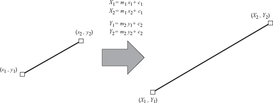
At the same time, the mapping y → Y is also linear represented as
Solving the first two equations, we obtain
The mapping equation in y → Y is solved in the same manner to produce the following results:
Equations (4.1) and (4.2) provide very useful conversion criteria of coordinates from Cartesian to Windows. The contribution is obvious especially in confining certain points in the real coordinate system to be within a rectangular region in Windows.
Example 4.1. The line from (−5, 6) to (7, −4) in the Cartesian coordinates system maps to a line from (50, 30) to (500, 300) in Windows. Find a line in Windows that is mapped from the line in the Cartesian system from (−2, 0) to (4, 2).
Solution. In this problem, (x1, y1) = (−5,6), (x2, y2) = (7, −4), (X1, Y1) = (50, 30), and (X2, Y2) = (500, 300). From Equations (4.3a), (4.3b), (4.4a), and (4.4b),

It follows that, X1 = 37.5(−2) + 237.5 = 162.5 ≈ 163, Y1 = −27(0) + 192 = 192, X2 = 37.5(4) + 237.5 = 387.5 ≈ 388 and Y2 = −27(2) + 192 = 138. Therefore, a line from (−2, 0) to (4, 2) in the Cartesian system maps directly to (163, 192) to (388, 138) in Windows.
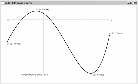
We discuss a small project called Code4B for drawing a polynomial on Windows. Figure 4.4 shows the polynomial f(x) = 2x4 + 2x3 − 9x2 − 4x + 1, which is the output of this project. The curve is drawn in the range of −1 ≤ x ≤ 1.8 with the maximum and minimum points as well as the left and right points of the curve shown. The coordinates shown are the real coordinates from the Cartesian system.
It is no secret that a curve is drawn on Windows by placing pixels successively through iterations from left to right according to its given function. In Code4B, the polynomial is produced by iterating the points (xi, yi) using the function yi = f(xi), for i = 0 to m, where x0 and xm are the left and right values, respectively, and m is the number of subintervals in the given range. Pixels are placed on the display using the MFC functions, SetPixel() or LineTo(). With large m, the successive pixels lie very close to each other so that they appear like a curve.
The main advantage from Code4B is the ease in which the polynomial is drawn according to scale on Windows. The drawing area in the window is bounded by a rectangle (not shown in the output) with the CPoint objects called home in the upper left-hand corner and end in the lower right-hand corner. With these defined boundaries, the curve is scaled in such a way that the maximum and minimum values touch the upper and lower boundaries of the rectangle. Therefore, the curve fits in nicely in the drawing area as it does not appear to be too big or too small this way.
Code4B is a brief project consisting of two files, Code4B.cpp and Code4B.h. Code4B.cpp is a relatively compact file consisting of about 100 lines of code. It has one class called CCode4B, which is derived from the MFC class, CFrameWnd. There is only one event in this project, namely, the main display, which is handled by the function OnPaint(). This implies Code4B does not take input from the user, and that most variables and objects are locally based.
In Code4B, the points in the Cartesian system with (x, y) real coordinates are declared in a structure called PT. The points along the curve are represented by an array called pt, which is linked to this structure, as follows:
typedef struct
{
      double x,y;
} PT;
PT *pt,max,min,left,right;
pt=new PT [m+1];
From this structure, the ith point in the graph is denoted as pt[i], with i = 0, 1, ..., m. The coordinates xi and yi of the point (xi, yi) are represented as pt[i].x and pt[i].y, respectively. Other members of this structure are left, right, min and max, which represent the left, right, minimum, and maximum points of the curve, respectively.
Figure 4.5 shows the drawing area of the curve on Windows showing the CPoint objects, home, end, left, right, max, and min. The drawing area is a rectangle designated by the CPoint objects, home (top left-hand corner) and end (bottom right-hand corner). With this designation, the drawing area for the curve is restricted to within the boundaries defined by the rectangle. A pixel in Windows is denoted px whose components, px.x and px.y, are the results from mapping pt[i].x and pt[i].y from the real coordinates according to Equations (4.1) and (4.2). This is illustrated in Figure 4.6. The left and right points of the curve in the given range are the CPoint objects, left and right. The maximum value of the curve is max, whereas its minimum is min.

Table 4.6 lists all the main variables in Code4B. There are m uniform subintervals in the x range whose width is given as h. Equations (4.1) and (4.2) convert the points from the real coordinates in the Cartesian system to their corresponding pixels in Windows with the constants determined by m1, c1, m2, and c2. The main objects in the project are listed in Table 4.7.
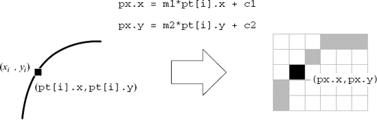
Table 4.6. The main variables in Code4B
Variable | Type | Description |
|---|---|---|
| double | (xi, yi) coordinates of a point in Cartesian. |
| double | Left point of the curve in the interval. |
| double | Right point of the curve in the interval. |
| double | Minimum point of the curve in the interval. |
| double | Maximum point of the curve in the interval. |
| double | Constants m1 and c1 from Equation (4.1). |
| double | Constants m2 and c2 from Equation (4.2). |
| double | Width of each subinterval. |
| macro | Total number of subintervals. |
Table 4.7. Main objects in Code4B
Object | Class | Description |
|---|---|---|
|
| Pixel on Windows with |
|
| Home (top left-hand corner) coordinates of the graphical area. |
|
| End (bottom right-hand corner) coordinates of the graphical area. |
In drawing the curve, the width of each subscriptinterval from x0 to xm is first computed, and this is given by
h=(pt[m].x-pt[0].x)/(double)m;
The curve is drawn by iterating on xi from i = 0 to i = m, incrementing the value of xi by h at each step. To determine the maximum and minimum values in the curve, comparisons are made through the expressions max.y<pt[i].y and min.y>pt[i].y, respectively. The following code segment shows how this is done:
max.y=0; min.y=0;
for (int i=0;i<=m;i++)
{
      pt[i].y=2*pow(pt[i].x,4)+2*pow(pt[i].x,3)
                  −9*pow(pt[i].x,2)−4*pt[i].x+1;
      if (max.y<pt[i].y)
            max=pt[i];
      if (min.y>pt[i].y)
            min=pt[i];
      if (i<m)
            pt[i+1].x=pt[i].x+h;
}
For mapping points from the real coordinates (pt[i].x,pt[i].y) into Windows coordinates (px.x,px.y), Equations (4.1) and (4.2) need to be solved. From Figure 4.5, we assign the variables in Equations (4.1) and (4.2) as follows:
x1 is | y1 is |
x2 is | y2 is |
X1 is | Y1 is |
X2 is | Y2 is |
Equations (4.4a) and (4.4b) then become
m1=(double)(end.x-home.x)/(pt[m].x-pt[0].x);
c1=(double)home.x-pt[0].x*m1;
m2=(double)(home.y-end.y)/(max.y-min.y);
c2=(double)end.y-min.y*m2;
In drawing a curve, it is important to have the x- and y-axes in the real coordinates shown for reference. These axes are drawn as follows:
CPen pGray(PS_SOLID,1,RGB(200,200,200));
dc.SelectObject(pGray);
px=CPoint(m1*0+c1,m2*min.y+c2); dc.MoveTo(px);
px=CPoint(m1*0+c1,m2*max.y+c2); dc.LineTo(px);
px=CPoint(m1*pt[0].x+c1,m2*0+c2); dc.MoveTo(px);
str.Format("%.0lf",pt[0].x); dc.TextOut(px.x,px.y,str);
px=CPoint(m1*pt[m].x+c1,m2*0+c2); dc.LineTo(px);
str.Format("%.1lf",pt[m].x); dc.TextOut(px.x,px.y,str);
The last step is to draw the curve by drawing points through iterations from left to right. The curve is drawn by moving the pen to pt[0], then drawing a line to the next point in the iteration, and so on until pt[m].x. Each point in the real coordinates pt[i] is mapped to its corresponding point on Windows px[i] using the conversion formula in Equations (4.1) and (4.2). At each iteration, comparisons are made to determine the maximum and minimum points of the curve. The following code shows how this is done:
CPen pDark(PS SOLID,2,RGB(50,50,50));
dc.SelectObject(pDark);
for (int i=0;i<=m;i++)
{
      px=CPoint((int)(m1*pt[i].x+c1), (int)(m2*pt[i].y+c2));
      if (i==0)
      {
            dc.MoveTo(px);
            str.Format("(%.2lf,%.4lf)",pt[0].x,pt[0].y);
            dc.TextOut(px.x,px.y,str);
      }
      else
            dc.LineTo(px);
      if (pt[i].y==max.y)
{
str.Format("(%.2lf,%.4lf)",max.x,max.y);
dc.TextOut(px.x,px.y-15,str);
}
if (pt[i].y==min.y)
{
str.Format("(%.2lf,%.4lf)",min.x,min.y);
dc.TextOut(px.x,px.y,str);
}
if (i<m)
pt[i+1].x=pt[i].x+h;
}
str.Format("(%.2lf,%.4lf)",pt[m].x,pt[m].y);
dc.TextOut(px.x,px.y-15,str);
dc.TextOut(100,350,"f(x)=2*x 4+2*x 3-9*x 2-4*x+1");
delete pt;The above code draws the curve perfectly in the given interval. Once this is done, it is important for us to delete the array pt from the structure as the allocated memory is still active although the program has ended. This is achieved through delete pt.
We have discussed Code4B for drawing a simple polynomial. The project illustrates some very important fundamental concepts in drawing a curve. However, the generated curve is static as the input is determined solely by the programmer. There is no flexibility as the end user will not get a chance to key in his/her own equations directly without the need to recompile the code. The program is also not user-friendly as there are no events associated with its interaction with the user.
A practical curve drawing program is one that allows interaction and has the user-friendliness features through MyParser. Curve drawing is considered complete if it incorporates an equation parser as one of its interactive tools. One useful application of an equation parser is in drawing a curve whose input equation is defined by the user. MyParser reads the equation keyed in by the user as a string, processes this string, and generates values for drawing the curve. We discuss two types of curves, namely, y = f (x), which is a curve that is dependent on a single variable x, and the parametric curve given by (x, y) = (f (t), g(t)).
The function y = f (x) is the most fundamental form of curve in mathematics. This function is a direct mapping from x to y through the relationship defined in f (x). This curve allows a single point in x to map to a point in y. It also allows several values of x to map to a single value in y. However, mapping a single point in x to multiple points of y is not allowed.
A parametric curve is a curve made up of points that are dependent on one or more parameters. A two-dimensional parametric curve represented by (x, y), where x and y are terms or functions that are dependent on the parameter t in the interval given by t0 ≤ t ≤ tm, is expressed as follows:
In a simple case like x = t and y = t2 for 0 ≤ t ≤ 2, the parametric equations are equivalent to a single equation given by y = x2, for 0 ≤ x ≤ 2. In some other cases, the relationship given by Equation (4.5) may not be expressed implicitly as a single function of x. For example, x = 2cost and y = 2 sin t are parametric equations representing a circle whose equation is x2 + y2 = 4.
We discuss Code4C, which provides flexibility by allowing the user to write an equation directly into an edit box. Figure 4.7 shows a sample output from quite a sophisticated function given by f(x) = 4 sin2x − 3 cos(1 − sinx) for −3 ≤ x ≤ 5. The parser in the program reads the expression keyed in by the user and computes the equation for i = 0 to m, where m is the number of intervals (which is also the number of iterations).
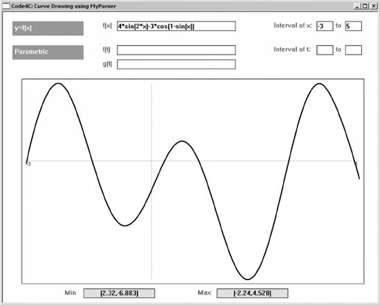
Code4C supports two types of graphs, the function y = f(x) and the parametric curve, x = f(t) and y = g(t). The two graphs can be selected using a menu in the form of shaded rectangular boxes. Input for the first type of graph is provided in the form of CEdit boxes that read the string for f(x) and range of values of x in the domain. For the second graph, CEdit input boxes are provided to read the strings x = f(t) and y = g(t) and the start and end values of t. The curve is shown in the big rectangular region, whereas its maximum and minimum points are displayed in the static boxes at the bottom of the window.
Figure 4.8 shows another example of a curve from a set of parametric equations given by x(t) = 1 + t cos t and y(t) = t sin(1 − t) for −30 ≤ t ≤ 50. In this example, the program determines the left and right values of x, as well as the maximum and minimum values of y from the given range of t. Creativity continues from here. The user should try several equations in mind and should view the results on the window.
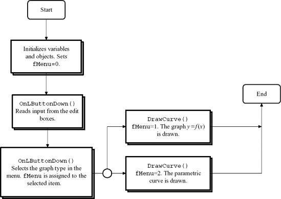
Figure 4.9 illustrates the development steps in Code4C. A global variable called fMenu has been created to monitor the progress in the execution, with fMenu = 0 as its initial value, and fMenu = 1 and fMenu = 2 indicating a selection of the first or second item in the menu, respectively. Input from the user in the edit boxes is read in OnLButtonDown(). Once input has been completed, a click at an item in the menu results in its assignment of value to fMenu. Another function called DrawCurve() draws the selected graph according to the input values.

Code4C includes three source files, Code4C.cpp, Code4C.h, and MyParser.obj. A single class called CCode4C is used, and this class is derived from CFrameWnd. The same structure called PT as in Code4B is used, but this time t is included as its additional member to support the parametric equations, x(t) and y(t). The structure is declared as follows:
typedef struct
{
      double t,x,y;         // x, y and t coordinates
} PT;
PT *pt,max,min,left,right;
The objects for the menu are organized into a structure called MENU. The structure consists of members that represent the title, home coordinates, and rectangular objects of the items. An array called menu[] stores these values.
typedef struct
{
      CString item;        // title
      CPoint hm;           // home coordinates
      CRect rc;            // rectangular object
} MENU;
MENU menu[nMenuItems+1];
Input is organized into a structure called INPUT.
typedef struct
{
      CString item;        // title
      CPoint hm;           // home coordinates
      CEdit ed;            // edit box
      CRect rc;            // rectangular object
} INPUT;
INPUT input[nInput+1];
Another structure is OUTPUT, which organizes the objects for displaying the output. The structure organizes objects for the static boxes and their home coordinates and rectangular objects through an array called output[].
typedef struct
{
      CPoint hm;        // home coordinates
      CStatic st;       // static box
      CRect rc;         // rectangular object
} OUTPUT;
OUTPUT output[nOutput+1];
The selected curve is displayed in the big rectangular region. A structure called CURVE organizes the objects comprising the starting and end coordinates of the rectangle and the rectangular object. This structure is linked to a variable called curve.
typedef struct
{
      CPoint hm,end;        // start and end coordinates
      CRect rc;             // rectangular object
} CURVE;
CURVE curve;
There are five main functions in Code4C, and they are listed in Table 4.8. OnPaint() responds to ON_WM_PAINT, which updates the output in the main window. A function called OnLButtonDown() responds to ON_WM_LBUTTONDOWN, which is immediately activated when an item in the menu is left-clicked. Another function, called DrawCurve(), draws and label the selected curve once input has been completed.
Table 4.8. Functions in Code4C
Function | Type | Description |
|---|---|---|
| Constructor | Creates the main window and initializes the variables and objects. |
| Destructor | Destroy the class and the array |
|
| Draw the curve selected from the menu. |
|
| Message handler for the left-click of the mouse. |
|
| Output display in the main window. |
Two events are mapped in this application, and they are the default display on the main window and the left-click of the mouse.
BEGIN_MESSAGE_MAP(CCode4C,CFrameWnd)
    ON_WM_PAINT()
    ON_WM_LBUTTONDOWN()
END_MESSAGE_MAP()
The code for the constructor function is listed below. Initial values are assigned to the global variables and objects. They include the home coordinates of all the menu items, edit and static boxes. The menu items are identified through a flag variable called fMenu, with fMenu=0 as its initial value to denote no selection has been made. The id for each edit and static boxes is uniquely assigned with the first box read given with an initial value of idc=301. To guarantee a unique id for each box, this value is incremented every time an edit box or static box is created.
CCode4C::CCode4C()
{
      int i;
      Create(NULL,"Code4C: Curve Drawing using MyParser",
            WS OVERLAPPEDWINDOW,CRect(0,0,800,640),NULL);
      pt=new PT [m+1];
      fMenu=0; idc=301;
      menu[1].item="y=f(x)";
      menu[2].item="Parametric";
      curve.hm=CPoint(50,150);
      curve.end=CPoint(750,560);
      curve.rc=CRect(curve.hm.x,curve.hm.y,curve.end.x,
            curve.end.y);
      input[1].hm=CPoint(240,20);
      input[2].hm=CPoint(660,20);
      input[3].hm=input[2].hm+CPoint(60,0);
input[4].hm=CPoint(660,70);
input[5].hm=input[4].hm+CPoint(60,0);
input[6].hm=input[1].hm+CPoint(0,50);
input[7].hm=input[6].hm+CPoint(0,30);
output[1].hm=CPoint(170,580);
output[2].hm=output[1].hm+CPoint(280,0);
for (i=1;i<=nMenuItems;i++)
{
menu[i].hm=CPoint(20,20+(i-1)*50);
menu[i].rc=CRect(menu[i].hm.x,menu[i].hm.y,
menu[i].hm.x+150,menu[i].hm.y+30);
}
for (i=1;i<=nOutput;i++)
output[i].st.Create("",WS_CHILD| WS_VISIBLE
| SS_CENTER|WS_BORDER,
CRect(output[i].hm.x,output[i].hm.y,
output[i].hm.x+150, output[i].hm.y+20),this,
idc++);
for (i=1;i<=nInput;i++)
input[i].ed.Create(WS CHILD|WS VISIBLE|WS BORDER,
CRect(input[i].hm.x,input[i].hm.y,
input[i].hm.x+((i>1 && i<6)?35:250),
input[i].hm.y+20), this,idc++);
Arial80.CreatePointFont (80,"Arial");
}OnPaint() displays the menu items and the labels for the edit boxes and static boxes. The function also updates the display in the main window and draws curve through DrawCurve() when it receives a call through InvalidateRect().
void CCode4C::OnPaint()
{
      CPaintDC dc(this);
      CString str;
      dc.SetBkColor(RGB(150,150,150));
      dc.SetTextColor(RGB(255,255,255));
      dc.SelectObject(Arial80);
      for (int i=1;i<=2;i++)
      {
            dc.FillSolidRect(&menu[i].rc,RGB(150,150,150));
            dc.TextOut(menu[i].hm.x+5,menu[i].hm.y+5,
                  menu[i].item);
      }
      CRect rc=CRect(curve.hm.x-10,curve.hm.y-10,curve.end.x+10,
            curve.end.y+10);
dc.Rectangle(rc);
dc.SetBkColor(RGB(255,255,255));
dc.SetTextColor(RGB(100,100,100));
dc.TextOut(input[1].hm.x-30, input[1].hm.y, "f(x)")
dc.TextOut(input[2].hm.x-90,input[2].hm.y,
"Interval of x:");
dc.TextOut(input[3].hm.x-20,input[3].hm.y,"to");
dc.TextOut(input[4].hm.x-90,input[4].hm.y,
"Interval of t:");
dc.TextOut(input[5].hm.x-20,input[5].hm.y,"to");
dc.TextOut(input[6].hm.x-30,input[6].hm.y,"f(t)");
dc.TextOut(input[7].hm.x-30,input[7].hm.y,"g(t)");
dc.TextOut(output[1].hm.x-40,output[1].hm.y,"Min");
dc.TextOut(output[2].hm.x-40,output[2].hm.y,"Max");
if (fMenu==1 || fMenu==2)
DrawCurve();
}The above code updates the display on certain parts of the window whenever the function InvalidateRect() is invoked. This is observed in the last two lines when fMenu is assigned with the value of 1 or 2 whenever a menu item is selected. The selection causes a curve to be drawn from the function DrawCurve().
OnLButtonDown() responds to ON_WM_LBUTTONDOWN. This happens whenanitem in the menu is left-clicked. This function has two parameters, nFlags and pxClick. We are only concerned with pxClick here as it represents an object for recording the pixel location where the click is made. OnLButtonDown() first reads the input made on the edit boxes through the MFC function, GetWindowText(). Each input is read as a string recognized as input[i].item. Inputs such as the left and right values of x are recognized as real values. Therefore, their input strings, input[2].item and input[3].item, respectively, are converted to double using the C++ function, atof(). Other inputs, input[1].item, input[6].item, and input[7].item, are global strings that represent the input expressions that will be read and evaluated by the parser.
void CCode4C::OnLButtonDown(UINT nFlags,CPoint pxClick)
{
      input[1].ed.GetWindowText(input[1].item);
      input[2].ed.GetWindowText(input[2].item);
      input[3].ed.GetWindowText(input[3].item);
      input[4].ed.GetWindowText(input[4].item);
      input[5].ed.GetWindowText(input[5].item);
      input[6].ed.GetWindowText(input[6].item);
      input[7].ed.GetWindowText(input[7].item);
      pt[0].x=atof(input[2].item);
pt[m].x=atof(input[3].item);
pt[0].t=atof(input[4].item);
pt[m].t=atof(input[5].item);
if (menu[1].rc.PtInRect(pxClick))
fMenu=1;
if (menu[2].rc.PtInRect(pxClick))
fMenu=2;
InvalidateRect(curve.rc);
}When a shaded rectangle in the window is left-clicked, pxClick stores the pixel coordinates at the location. A MFC function called PtInRect() checks whether the click is within the named rectangle. For example, the following expression checks whether if the first box has been clicked:
menu[1].rc.PtInRect(pxClick)
where menu[1].rc is the rectangle and pxClick is the location of the click. The function returns TRUE (1) if the click is inside the rectangle, and FALSE (0) if it is outside of the rectangle. A return value of 1 validates the selection, and the program immediately assigns fMenu to indicate the type of function chosen.
The last statement in OnLButtonDown() updates the display in the main window. This is done through InvalidateRect(), which calls OnPaint() for updating a rectangular region in the display denoted by curve.rc.
The most important content in Code4C is the function for drawing a curve, DrawCurve(). The code of this function is derived mostly from a function of the same name in Code4B with some enhancement from the parser. The parser incorporates a function called parse(), which is derived from the external object file, MyParser.obj. This external function is called through the statement
extern double parse(CString,int,double [],int []);
in the header file.
DrawCurve() draws a curve based on the assigned value assigned to fMenu, where fMenu=1 indicates the curve y = f (x) and fMenu=2 for the parametric curve. The first curve is drawn according to the following code segment:
if (fMenu==1)
{
      h=(pt[m].x-pt[0].x)/((double)(m));
      for (i=0;i<=m;i++)
      {
            psi[1]=23; psv[1]=pt[i].x;
            pt[i].y=parse(input[1].item,1,psv,psi);
if (i==0)
{
left.x=0; right.x=0;
min=pt[0]; max=pt[0];
}
left.x=((left.x>pt[i].x)?pt[i].x:left.x);
right.x=((right.x<pt[i].x)?pt[i].x:right.x);
if (min.y>pt[i].y)
{
min.x=pt[i].x; min.y=pt[i].y;
}
if (max.y<pt[i].y)
{
max.x=pt[i].x; max.y=pt[i].y;
}
if (i<m)
pt[i+1].x=pt[i].x+h;
}
}The above code computes yi = f (xi) for i = 0, 1, ..., m. The code also determines the maximum and minimum points in the curve as well as the left and right intervals for x. The x variable is identified as a code in psi[1]=23. The value assigned to this variable is stored as psv[1]. These two values make up the arguments in parse(), which reads the string expression from input[1].item, as follows:
pt[i].y=parse(input[1].item,1,psv,psi);
The entry of 1 in the above statement denotes only one variable is involved in the expression. The above statement computes the expression in input[1].item and returns the value as pt[i].y.
The second type of curve is generated from fMenu=2. Two variables are involved, t and x, and they are identified as codes 19 and 23, respectively. The first function in this parametric equation, x = f (t), is evaluated from the global string through
psi[1]=19; psv[1]=pt[i].t;
pt[i].x=parse(input[6].item,1,psv,psi);
The second function y = g(t) is read as input[7].item and evaluated through
psi[1]=23; psv[1]=pt[i].x;
pt[i].y=parse(input[7].item,1,psv,psi);
The following code segment evaluates xi = f (ti) and yi = g(ti) for i = 0, 1, ..., m besides determining the maximum, minimum, left, and right points in the curve:
if (fMenu==2)
{
      h=(pt[m].t-pt[0].t)/((double)(m));
      for (int i=0;i<=m;i++)
      {
            psi[1]=19; psv[1]=pt[i].t;
            pt[i].x=parse(input[6].item,1,psv,psi);
            psi[1]=23; psv[1]=pt[i].x;
            pt[i].y=parse(input[7].item,1,psv,psi);
            if (i==0)
            {
                  left.x=0; right.x=0;
                  min=pt[0]; max=pt[0];
            }
            left.x=((left.x>pt[i].x)?pt[i].x:left.x);
            right.x=((right.x<pt[i].x)?pt[i].x:right.x);
            if (min.y>pt[i].y)
            {
                  min.x=pt[i].x; min.y=pt[i].y;
            }
            if (max.y<pt[i].y)
            {
                  max.x=pt[i].x; max.y=pt[i].y;
            }
            if (i<m)
                  pt[i+1].t=pt[i].t+h;
      }
}
With all computed values for (xi, yi) determined from the parser, the last step in the project is to display the curve in the designated graphical region. This is done through
CPen pDark(PS SOLID,2,RGB(50,50,50));
dc.SelectObject(pDark);
for (i=0;i<=m;i++)
{
      px=CPoint((int)(m1*pt[i].x+c1), (int)(m2*pt[i].y+c2));
      if (i==0)
            dc.MoveTo(px);
      else
            dc.LineTo(px);
}In this chapter, we discussed in detail the techniques for drawing several types of curves on Windows using the resources in MFC. As the platforms on Windows and the real coordinates in mathematics differ, some simple transformations are required to make them compatible. In addition, we also discussed MyParser, which is a very useful tool in <mathematics for developing user-friendly mathematical applications. MyParser incorporates an equation parser that reads and evaluates a mathematical equation from the user in the form of a string. The user should find the supplied object file in MyParser very useful as this file can be linked to other source files in a project for solving many numeric-intensive applications. Some useful applications include the final year undergraduate, M.Sc, and Ph.D. projects, and modeling and simulation in research.
Test on the following curves using
Code4B:y = 1 − 3x + 5x2.
y = 3x sinx − 5x2 cos(1 − x).

x(t) = 2 cos(2t − 1) and y(t) = t sin(t2 − 1).
x(t) = 3 sin2t and y = 3 cos2t.
The polar coordinate system is represented as r = f(θ), where r is the radius from the origin and θ is the angle measured from the x-axis in the counter-clockwise direction. The conversion from (r, θ) to (x, y) is done according to the following rules:
x = r cos θ and y = r sin θ. Improve on the program in
Code4Ato include a polar curve given by r = sin 5θ.Improve on the program in
Code4Cto include equations from the polar coordinates.The curve drawing project in
Code4Cdoes not include mechanisms for checking the domain of the function and for testing for its singularity at the points in the given interval. These issues are important to consider as they may cause the program to crash if not handled carefully. Study these issues, and incorporate them intoCode4C.