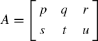
Engineering problems involving large arrays with high-resolution graphics for visualization are some of the typical applications in high-performance computing. In most cases, high-performance computing is about intensive numerical computing over a large problem that requires good accuracy and high-precision results. High-performance computing is a challenging area requiring advanced hardware as well as a nicely crafted software that makes full use of the resources in the hardware.
Numerical applications often involve a huge amount of computation that requires a computer with fast processing power and large memory. Fast processing capability is necessary for calculating and updating several large size arrays, which represent the computational elements of the numerical problem. Large memory is highly desirable to hold the data, which also contributes toward speeding up the calculations.
C++ was originally developed in the early 1980s by Bjarne Stroustrup. The features in C++ have been laid out according to the specifications laid by ANSI (American National Standards Institute) and ISO (International Standards Organization). The language is basically an extension of C that was popular in the 1970s, replacing Pascal and Fortran. C is a highly modular and structured high-level language, which also supports low-level programming. The language is procedural in nature, and it has what it takes to perform numerical computing besides being used for general-purpose applications, such as in systems-level programming, string processing, and database construction.
Primarily, C++ extends what is lacking in C, namely, the object-oriented approach to programming, for supporting today's complex requirements. Object-oriented programming requires a problem to be broken down into objects, which can then be handled in a more practical and convenient manner. That is the standard put forward for meeting today's challenging requirements. The programming language must provide support for exploring the computer's resources in providing an easy and friendly-looking graphical user interface for the given applications. The resources are provided by the Windows operating system, which includes the mouse's left and right button clicks, text and graphics, keys from the keyboard, dialog boxes, and multimedia support. In addition, C++ is a scalable language that makes possible the extension of the language to support several new requirements, for meeting today's requirements, including the Internet, parallel computing, wireless computing, and communication with other electronic devices.
In performing scientific computing, several properties for good programming help in achieving efficient coding. They include
In this chapter, we discuss several fundamental mathematical tools and their programming strategies that are commonly deployed in high-performance computing. They include strategies for allocating memory dynamically on arrays, passing array data between functions, performing algebraic computation on complex numbers, producing random numbers, and performing algebraic operations on matrices. As the names suggest, these tools provide a window of opportunity for high performance computing that involves vast areas of numeric-intensive applications.
A variable represents a single element that has a single value at a given time. An array, in contrast, is a set of variables sharing the same name, where each of them is capable of storing one value at a single time. An array in C++ can be in the form of one or more dimensions, depending on the program requirement. An array is suitable for storing quantities such as the color pixel values of an image, the temperature of the points in a rectangular grid, the pressure of particles in the air and the values returned by sensors in an electromagnetic field.
An array is considered large if its size is large. One typical example of large arrays is one that represents an image. A fine and crisp rectangular image of size 1 MB produced from a digital camera may have pixels formed from hundreds of rows and columns. Each pixel in the image stores an integer value representing its color in the red, green, and blue scheme.
A computer program having many large arrays often produces a tremendous amount of overhead to the computer. The speed of execution of this program is very much affected by the data it carries as each array occupies a substantial amount of memory in the computer. However, a good strategy for managing the computer's memory definitely helps in overcoming many outstanding issues regarding large arrays. One such strategy is dynamic memory allocation where memory is allocated to arrays only when they are active and is deallocated when they are inactive.
In scientific computing, a set of variables that have the same dimension and length is often represented as a single vector. Vector is an entity that has magnitude or length and direction. Opposite to that is a scalar, which has magnitude but does not have direction. For example, the mass of an object is a scalar, whereas its weight subject to the gravitational pull toward the center of the earth is a vector.
In programming, a vector is represented as a one-dimensional array. A vector v of size N has N elements defined as follows:

The above vector is represented as a one-dimensional array, as follows:
V[1],V[2],...,V[N].
The magnitude or length of this vector is

In numerical applications, this vector can be declared as real or integer depending on the data it carries. The length of the vector needs to be declared as a floating-point as the value returned involves decimal points. It is important to declare the variable correctly according to the variable data type as wrong declaration could result in data loss.
As the size of an array can reach several hundreds, thousands, or even millions, an optimum mechanism for storing its data is highly desirable. For a small size array, static memory allocation is a normal way of storing the data. An array v with N+1 elements is declared statically as
int v[N+1];
This array consists of the elements v[0], v[1], ..., v[N], and memory from the computer's RAM has been set aside for this array no matter whether all elements in the array are active. Having only v[1], v[2], and v[3] active out of N = 100 from the above declaration is clearly a waste as memory has been allocated to all 100 elements in the array. This mode of allocating memory is called static memory allocation.
A more practical way of allocating memory is the dynamic memory allocation where memory from the computer is allocated to the active elements only in the array.
In dynamic memory allocation, the same array whose maximum size is N+1 is declared as follows:
int *v;
v=new int v[N+1];
Memory for a one-dimensional array is allocated dynamically as a pointer using the new directive. The allocated size in the declaration serves as the upper limit; memory is allocated according to the actual values assigned to the elements in the array. For example, the array v above is allocated with a maximum of N+1 elements, but memory is assigned to three variables that are active only, as follows:
int *v; //declaring a pointer to theinteger arrayv = new int [N+1]; //allocating memory of size N+1v[1]=7; v[2]=−3; v[3]=1; //assigning values to the array... ... delete v; //destroying the array
Once the array has completed its duty and is no longer needed in the program, it can be destroyed using the delete directive. The destruction means the array can no longer be used, and the memory it carries is freed. In this way, the memory can be used by other modules in the program, thus, making the system healthier.
Dynamic memory allocation for one-dimensional arrays is illustrated using an example in multiplying two vectors. The multiplication or dot product of two vectors of the same size n, u = [u1 u2 ... uN] T and v = [v1 v2 ... vN] T produces a scalar, as follows:
This task is implemented in C++ with the result stored in w in the following code:
w=0;
for (i=1;i<=N;i++)
         w += u[i]*v[i];
The above code has a complexity of O(N). Code2A.cpp shows a full C++ program that allocates memory dynamically to the one-dimensional arrays u and v, and it computes the row product between the two arrays:
Code2A.cpp: dot-product of two vectors
#include <iostream.h>
#define N 3
void main()
{
     int i;
     int *u, *v, w;
     u=new int [N+1];
     u[1]=4; u[2]=−5; u[3]=3;
     cout << endl << "Vector u:" << endl;
     for (i=1;i<=N;i++)
           cout << u[i] << " ";
     cout << endl;

     v=new int [N+1];
     v[1]=−2; v[2]=3; v[3]=7;
     cout << "Vector v:" << endl;
     for (i=1;i<=N;i++)
           cout << v[i] << " ";
     cout << endl;

     w=0;
     for (i=1;i<=N;i++)
           w += u[i]*v[i];
     cout << "the product w=u.v is " << w << endl;
     delete u,v;
}A two-dimensional array represents a matrix that consists of a set of vectors placed as its columnar elements. Basically, a two-dimensional array q with M+1 rows and N+1 columns is declared as follows:
int q[M+1][N+1];
The above declaration is the static way of allocating memory to the array. The dynamic memory allocation method for the same array is shown, as follows:
int **q; //declaring a pointer to theinteger arrayq = new int *[M+1]; //allocating memory of sizeM+1 to the rowsfor (int i=0;i<=M;i++)
q[i]=new int [N+1];// allocating memory of sizeN+1 to the columns... ... for (i=0;i<=N;i++) delete q[i]; //deallocating the columnararray memorydelete q; //destroying the array
In the above method, a double pointer to the variable is needed because the array is two-dimensional. Memory is first allocated to the M+1 row vectors in q. Each row vector has N+1 columns, and therefore, another chunk of memory is allocated to each of these vectors. Hence, a maximum total of [M+1][N+1] amount of memory is allocated to this array.
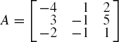
We illustrate an important tool in linear algebra involving the multiplication of two matrices whose memories are allocated dynamically. Suppose A = [aik] and B = [bkj] are two matrices with i = 1, 2, ..., M representing the rows of A, and j = 1, 2, ..., N are the columns in B. The basic rule allowing two matrices to be multiplied is the number of columns in the first matrix must be equal to the number of rows of the second matrix, which is k = 1, 2, ..., P. The product of A and B is then matrix C = [cij], or
AB = C.
For example, if A and B are matrices of size 3 × 4 and 4 × 2, respectively, then their product is matrix C with the size of 3 × 2, as follows:

Obviously, each element in the resultant matrix is the sum of four terms that can be written in a more compact form through their sequence. For example, c11 has the following entry:
which can be rewritten in a simplified form as

Other elements can be expressed in the same general manner. The elements in matrix C become

Looking at the sequential relationship between the elements, the following simplified expression represents the overall solution to the matrix multiplication problem:

for i = 1, 2, ..., M, and j = 1,2, ..., N. This compact form is also the algorithmic solution for the matrix multiplication problem as program codes can easily be designed from the solution.
We discuss the program design for the above problem. Three loops with the iterators i, j, and k are required. As k is the common variable representing both the row number of A and the column number of B, it is ideally placed in the innermost loop. The middle loop has j as the iterator because it represents the column number of C. The outermost loop then represents the row number of C, having i as the iterator.
The corresponding C++ code for the multiplication problem has the complexity of O(MNP), and the code segments are
for (i=1; i<=M; i++)
      for (j=1; j<=N; j++)
      {
             c[i][j]=0;
             for (k=1; k<=P; k++)
                   c[i][j] += a[i][k]*b[k][j];
      }
Code2B.cpp is a full program for the multiplication problem between the matrices A = [aik] and B = [bkj] with i = 1, 2,..., M and j = 1, 2,..., N. The program demonstrates the full implementation of the dynamic memory allocation scheme for two-dimensional arrays.
Code2B.cpp: multiplying two matrices
#include <iostream.h>
#define M 3
#define P 4
#define N 2

void main()
{
     int i,j,k;
     int **a,**b,**c;
     a = new int *[M+1];
     b = new int *[P+1];
     c = new int *[M+1];
     for (i=1;i<=M;i++)
           a[i]=new int [P+1];
     for (j=1;j<=P;j++)
           b[j]=new int [N+1];
     for (k=1;k<=M;k++)
           c[k]=new int [N+1];

     a[1][1]=2; a[1][2]=−3; a[1][3]=1; a[1][4]=5;
     a[2][1]=−1; a[2][2]=4; a[2][3]=−4; a[2][4]=−2;
     a[3][1]=0; a[3][2]=−3; a[3][3]=4; a[3][4]=2;
     cout << "Matrix A:" << endl;
     for (i=1; i<=M; i++)
     {
           for (j=1;j<=P;j++)
                 cout << a[i][j] << " ";
           cout << endl;
     }

     b[1][1]=4; b[1][2]=−1;
     b[2][1]=3; b[2][2]=2;
     b[3][1]=1; b[3][2]=−1;
     b[4][1]=−2; b[4][2]=4;
     cout << endl << "Matrix B:" << endl;
     for (i=1; i<=P; i++)
     {
           for (j=1; j<=N; j++)

                 cout << b[i][j] << " ";
cout << endl;
}
cout << endl << "Matrix C (A multiplied by B):" << endl;
for (i=1; i<=M; i++)
{
for (j=1;j<=N;j++)
{
c[i][j]=0;
for (k=1;k<= P;k ++)
c[i][j] += a[i][k]*b[k][j];
cout << c[i][j] << " ";
}
cout << endl;
}
for (i=1;i<=M;i++)
delete a[i];
for (j=1;j<=P;j++)
delete b[j];
for (k=1;k<=M;k++)
delete c[k];
delete a,b,c;
}The declaration and coding for arrays with higher dimensions in dynamic memory allocation follow a similar format as those in the one- and two-dimensional arrays. For example, a three-dimensional array is declared statically as follows:
int r[M+1][N+1][P+1];
The following code shows the dynamic memory allocation method for the same array:
int ***r; //declaring a pointerto the integer arrayr = new int **[M+1]; //allocation to thefirst parameterfor (int i=0;i<=M;i++) { r[i]=new int *[N+1]; //allocation to thesecond parameterfor (int j=0;j<=N;j++) r[i][j]=new int [P+1]; //allocation to thethird parameter} ...
...

for (i=0;i<=N;i++)
{
     for (j=0;j<=P;j++)
           delete r[i][j];
     delete r[i];
}
delete r; // destroying the arrayOne of the most important operations involving a matrix is its reduction to the upper triangular form U. The technique is called row operations, and it has a wide range of useful applications for solving problems involving matrices. Row operation is an elimination technique for reducing a row in a matrix into its simpler form using one or more basic algebraic operations from addition, subscripttraction, multiplication, and division. A reduction on one element in a row must be followed by all other elements in that row in order to preserve their values.
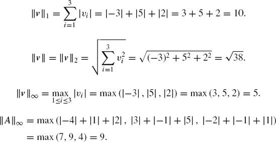
The norm of a vector is a scalar value for describing the size or length of the vector with respect to the dimension n of the vector. Norm values of a vector are extensively referred especially in evaluating the errors that arise from an operation involving the vector.
Definition 2.1. The norm-n of a vector of size m, v = [v1 v2 ... vm] T, is defined as the nth root of the sum to the power of n of the elements in the vector, or

It follows from Definition 2.1 that the first norm of v = [v1 v2 ... vn] T, called the sum of the vector magnitude norm, is the sum of the absolute value of the elements, as follows:

The second norm of v = [v1 v2 ... vm] T is called the Euclidean vector norm, which is expressed as follows:

Another important norm is the maximum vector magnitude norm, or || v ||∞ of v = [v1 v2 ... vm]T, which is the maximum of the absolute value of the elements. This norm is defined as follows:
The rule for determining the maximum matrix norm follows from that of a vector because a matrix of size m × n is made up of m rows of n column vectors each. This is expressed as follows:

Example 2.1. Given v = [−3, 5, 2]T and
Solution. The calculation is very straightforward, as follows:
Row operations are the key ingredients for reducing a given matrix into a simpler form that describes the behavior and properties of the matrix.
Definition 2.2. Row operation on row i with respect to row j is an operation involving addition and substraction defined as Ri ← Ri + m Rj, where m is a constant and Ri denotes row i. In this definition, Ri on the left-hand side is a new value obtained from the update with Ri on the right-hand side as its old value.
Theorem 2.1. Row operation in the form Ri ← Ri + m Rj on row i with respect to row j does not change the matrix values. In this case, the matrix with the reduced row is said to be equivalent to the original matrix.
Consider matrix
The addition operation on R2 produces

From Theorem 2.1, the new matrix obtained, B, is said to have equal values with the original matrix A. Another operation is substraction:

which results in matrix C having the same values as A and B. We say all three matrices are equivalent, or

A useful reduction is the case in which the constant m is based on a pivot element. A pivot element is an element in a row that serves as the key to the operation on that row. The normal goal of pivoting an element is to reduce the value of an element to zero. In matrix C above, the element a21 in A can be reduced to 0 by letting

Reduction to zero elements is the basis of a technique for reducing a matrix to its triangular form. A triangular matrix is a square matrix where all elements above or below the diagonal elements have zero values. The name triangular is reflected in the shape of the matrix with two triangles occupying the elements, one with zero elements of the matrix and another with other numbers (including zeros).
An upper triangular matrix is a triangular matrix denoted as U = [uij], where uij = 0 for j < i. Other elements with j ≥ i can have any value including zero. For example, a 4 × 4 upper triangular matrix has the following form:
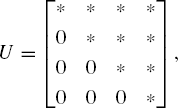
where * can be any number including 0.
Opposite to the upper triangular matrix is the lower triangular matrix L = [lij], where lij = 0 for i < j. The following matrix is a general notation for the 4 × 4 lower triangular matrix L:

A square matrix A is reduced to U or L through a series of row operations. Row operation is a technique for reducing a row in a matrix into a simpler form by performing an algebraic operation with another row in the matrix. Matrix A, when reduced to U or L, is said to be equivalent to that matrix.
In general, a square matrix with N rows requires N − 1 row operations with respect to rows 1, 2, ..., N − 1. A matrix is usually reduced by eliminating all the rows of one of its columns to zero with respect to the pivot element in the row. The pivot elements of matrix A = [aij] are aii, which are the diagonal elements of the matrix. The reduction of a square matrix into its upper triangular matrix is best illustrated through a simple example.
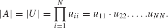
Example 2.2. Find the upper triangular matrix U of the following matrix:

Solution. There are four rows in the matrix. Reduction of the matrix to its upper triangular form requires three row operations with respect to rows 1, 2, and 3.
Operations with Respect to the First Row. a11 = 8.000 is the pivot element of the first row, and let m = ai1/a11 for the rows i = 2, 3, 4. All elements in the second, third, and fourth rows are reduced to their corresponding values using the relationships aij ← aij − m*a1j for columns j = 1, 2, 3, 4.

Operations with Respect to the Second Row. a22 = 1.500 is the pivot element of the second row, and therefore, m = ai2/a22 for the rows i = 3, 4. All elements in the third and fourth rows are reduced to their corresponding values using the relationships aij ← aij − m*a2j for the columns j = 1, 2, 3,4.
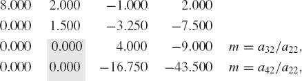
Operations with Respect to the Third Row. a33 = 4.000 is the pivot element of the third row. Therefore, m = ai3/a33 for the row i = 4. All elements in the fourth row are reduced to their corresponding values using the relationship aij ← aij − m*a3j for the columns j = 1, 2, 3,4.

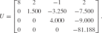
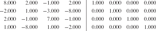
Row operations on A produce U:
The C++ program to reduce A to U is very brief and compact. The code is constructed from the equation aij ← aij − m*akj, where m = aik/akk, and i = k + 1, k + 2, ..., N, k = 1, 2,..., N − 1 and j = 1, 2,..., N, as follows:
double m;
for (k=1;k<=N-1;k++)
        for (i=k+1;i<=N;i++)
{
m=a[i][k]/a[k][k];
for (j=1;j<=N;j++)
a[i][j] -= m*a[k][j];
}Code2C.cpp shows the full program for reducing A to U with Code2C. in as the input tile for A
Code2C.cpp: reducing a square matrix to its upper triangular form
#include <fstream.h>
#include <iostream.h>
#define N 4
void main()
{
int i,j,k;
double **a;
a=new double *[N+1];
for (i=0;i<=N;i++)
a[i]=new double [N+1];
ifstream InFile("Code2C.in");
for (i=1;i<=N;i++)
for (j=1;j<=N;j++)
InFile >> a[i][j];
InFile.close();
// row operations
double m;
for (k=1;k<=N-1;k++)
for (i=k+1;i<=N;i++)
{
                m=a[i][k]/a[k][k];
                for (j=1;j<=N;j++)
                        a[i][j] -= m*a[k][j];
        }
for (i=1;i<=N;i++)
{
for (j=1;j<=N;j++)
cout << a[i][j] << " ";
cout << endl;
}
}As we will see later, the triangular form of a matrix says a lot about the properties of its original matrix, which includes the determinant of the matrix. Finding the determinant of a matrix proves to be an indispensable tool in numerical computing as it contributes toward determining some properties of the matrix. This includes an important decision such as whether the inverse of the matrix exists.
Definition 2.3. The determinant of a matrix A = [aij] can only be computed if it is a square matrix and A is reducible to U.
Definition 2.4. A square matrix A = [aij] is said to be singular if its determinant is zero. Otherwise, the matrix is nonsingular. A singular matrix is not reducible to U.
Definition 2.5. The inverse of a singular matrix does not exist, which implies that if A is nonsingular, then its inverse, or A−1, exists.
The determinant of matrix A, denoted by |A| or det(A), is computed in several different ways. By definition, the determinant is obtained by computing the cofactor matrix from the given matrix. This method is easy to implement, but it requires many steps in its calculations.
A more practical approach to computing the determinant of a matrix is to reduce the given matrix to its upper or lower triangular matrix based on the same elimination method discussed above.
Theorem 2.2. If a square matrix is reducible to its triangular matrix, the determinant of this matrix is the product of the diagonal elements of its reduced upper or lower triangular matrix.
The above theorem states that if a square matrix A = [aij] of size N × N is reducible to its upper triangular matrix U = [uij], then
Example 2.3. Find the determinant of the matrix defined in Example 2.2.
Solution. From Theorem 2.2, the determinant of matrix A in Example 2.2 is the product of the diagonal elements of matrix U, as follows:

The following code shows how a determinant is computed:
double Product, m;
for (k=1;k<=N-1;k++)
      for (i=k+1;i<=N;i++)
      {
            m=a[i][k]/a[k][k];
            for (j=1;j<=N;j++)
                 a[i][j] -= m*a[k][j];
      }
Product=1;
for (i=1;i<=N;i++)
       Product *= a[i][i];
The full program for computing the determinant of a square matrix is listed in Code2D.cpp, as follows:
Code2D.cpp: computing the determinant of a matrix
#include <fstream.h>
#include <iostream.h>
#define N 4

void main()
{
     int i,j,k;
     double A[N+1][N+1];

     cout.setf(ios::fixed);
     cout.precision(5);
     cout << "Input matrix A: " << endl;
     ifstream InFile("Code2D.in");
     for (i=1;i<=N;i++)
     {
            for (j=1;j<=N;j++)
            {
                 InFile >> A[i][j];
                 cout << A[i][j] << " ";
            }
            cout << endl;
     }
     InFile.close();

     // row operations
     double Product,m;
     for (k=1;k<=N-1;k++)
            for (i=k+1;i<=N;i++)
{
m=A[i][k]/A[k][k];
for (j=1;j<=N;j++)
A[i][j]-=m*A[k][j];
}
cout << endl << "matrix U:" << endl;
for (i=1;i<=N;i++)
{
for (j=1;j<=N;j++)
cout << A[i][j] << " ";
cout << endl;
}
Product=1;
for (i=1;i<=N;i++)
Product *= A[i][i];
// display results
cout << endl << "det(A)=" << Product << endl;
}Finding the inverse of a matrix is a direct application of the row operations in the elimination method described earlier. Therefore, the problem is very much related to the row operations in reducing a given square matrix into its triangular form.
Theorem 2.3. The inverse of a square matrix A is said to exist if the matrix is not singular, that is, if its determinant is not zero, or |A| ≠ 0.
The above theorem specifies the relationship between the inverse of a square matrix and its determinant. The product of a matrix A and its inverse A−1 is AA−1 = I, where I is the identity matrix. Hence, the problem of finding the inverse is equivalent to finding the values of matrix X in the following equation:
AX = I.
X from the above relationship can be found through row operations by defining an augmented matrix A|I. Row operations reduce A on the left-hand side to U and I on the right-hand side to a new matrix V. Continuing the process, U on the left-hand side of the augmented matrix is further reduced to I, whereas V on the right-hand side becomes X = A−1, which is the solution.
Figure 2.1 depicts the row operations technique for finding the inverse of the matrix A. It follows that Example 2.3 illustrates an example in implementing this idea.

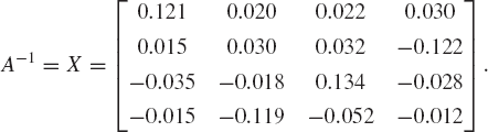
Example 2.4. Find the inverse of the matrix in Example 2.2.
Solution. The first step in solving this problem is to form the augmented matrix A | I, as follows:
Operations with Respect to Row 1. Start the operations with respect to row 1 with m = ai1/a11 by reducing a21, a31 and a41 to 0 through the equations aij ← aij − m*a1j and xij ← xij − m*x1j for the columns j = 1, 2, 3, 4.

Operations with Respect to Row 2. The next step is row operations with respect to row 2 with m = ai2/a22 for i = 3, 4 to reduce a32 and a42 to 0. This is achieved through aij ← aij − m*a2j and xij ← xij − m*x2j for the columns j = 1, 2, 3, 4, to produce the following values:

Operations with Respect to Row 3. Finally, U is produced from row operations with respect to row 3 with m = ai3/a33 for i = 4. Other elements in the row are updated according to aij ← aij − m*a3j and xij ← xij − m*x3j for j = 1, 2, 3, 4.

Reducing U to I. The next step is to reduce U from the left portion of the augmented matrix to the identity matrix I. The strategy is perform row operations starting on row 4 to reduce aj4 to 0 for j = 1, 2, 3, 4.

This is followed by row operations with respect to row 3.

The next step is the row operations with respect to row 2.
The last step is to reduce the diagonal matrix into an identity matrix by dividing each row with its corresponding diagonal element, as follows:

We obtain the solution matrix
The following program, Code2E.cpp, is the implementation of the elimination method for finding the inverse of a matrix.
Code2E.cpp: finding the inverse of a matrix
#include <fstream.h>
#include <iostream.h>
#define N 4

void main()
{
      int i,j,k;
      double **A, **B, **X;
      A=new double *[N+1];
      B=new double *[N+1];
      X=new double *[N+1];
      for (i=0;i<=N;i++)
      {
            A[i]=new double [N+1];
            B[i]=new double [N+1];
            X[i]=new double [N+1];
      }
cout.setf(ios::fixed);
cout.precision(5);
ifstream InFile("Code2E.in");
for (i=1;i<=N;i++)
for (j=1;j<=N;j++)
{
InFile >> A[i][j];
if (i==j)
B[i][j]=1;
else
B[i][j]=0;
}
InFile.close();
// row operations
double Sum,m;
for (k=1;k<=N-1;k++)
for (i=k+1;i<=N;i++)
{
m=A[i][k]/A[k][k];
for (j=1;j<=N;j++)
{
A[i][j] -= m*A[k][j];
B[i][j] -= m*B[k][j];
}
}
// backward subscriptstitutions
for (i=N;i>=1;i--)
for (j=1;j<=N;j++)
{
Sum=0;
for (k=i+1;k<=N;k++)
Sum += A[i][k]*X[k][j];
X[i][j]=(B[i][j]-Sum)/A[i][i];
}
for (i=1;i<=N;i++)
{
for (j=1;j<=N;j++)
cout << X[i][j] << " ";
cout << endl;
}
}Mathematical operations involving matrices can be very tedious and time consuming. This is especially true as the size of the matrices become large. As described, each matrix in a typical engineering application may occupy a large amount of computer memory. As a result, a mathematical operation involving several large matrices may slow down the computer and may cause the program to hang because of insufficient memory.
Efficient coding is required to handle algebraic operations involving many matrices. The preparation for a good coding includes the use of several functions to make the program modular and a distance separation of code from its data. The two requirements mean a good C++ program must implement an extensive data passing mechanism between functions as a way to simplify the execution of code.
Generally, algebraic operations on matrices involve all four basic tools: addition, subscripttraction, multiplication, and division. We discuss all four operations and our preparation for the large-scale algebraic operations. In achieving these objectives, we discuss methods for passing data between functions that serve as an unavoidable mechanism in making the program modular.
In making the program modular, several functions that represent the modules in the problem are created. Four main functions in matrix algebra are addition (with substraction), multiplication, and matrix inverse (which indirectly represents matrix division). We discuss the modular technique for solving an algebraic operation involving matrices based on all of these primitive operations. To simplify the discussion, all matrices discussed are assumed to be square matrices of the same size and dimension.
A good computer program considers data and program code as separate entities. In most cases, data should not be a part of the program. Data should be stored in an external storage medium, and it will only be called when required. This strategy is necessary as each unit of data occupies some precious space in the computer memory.
Data passing is important in making the program modular. Data passing encourages the variables to be declared locally instead of globally. A good C++ program should promote the use of local variables as much as possible in place of global variables as this contributes to the modularity of the program significantly. For example, if A is the input matrix for the addition function in a program, this same matrix should also be the input for the multiplication function. It is important to have a mechanism to allow data from the matrix to be passed from one function to another.
Two matrices of the same dimension, A = [aij] and B = [bij] are added to produce a new matrix C = [cij], which also has the same dimension as the first two matrices. The matrix addition between two matrices is a straightforward addition between the elements in the two matrices; that is, cij = aij + bij. The task is represented as the function MatAdd() from a class called MatAlgebra, as follows:
void MatAlgebra::MatAdd(bool flag,double **c,double **a,
     double **b)
{
     int i,j,k;
     for (i=1;i<=N;i++)
           for (j=1;j<=N;j++)
                 if (flag)
                        c[i][j]=a[i][j]+b[i][j];
                 else
                        c[i][j]=a[i][j]-b[i][j];
}
In MatAdd(), the input matrices are a and b, which receive data from the calling function. The computed array is c, which returns the value to the calling function in the program. The Boolean variable, flag, is introduced in the code to allow the function to support subscripttraction as well as addition. Addition is performed when flag=1 (TRUE), whereas flag=0 (FALSE) means subscripttraction. The use of flag is necessary to avoid the creation of another function specifically for, substraction, which proves to be redundant.
The matrix multiplication function is another indispensable module in matrix algebra. We call the function MatMultiply(), and its contents are very much similar to Code2B.cpp, as follows:
void MatAlgebra::MatMultiply(double **c,double **a, double **b)
{
     int i,j,k;
     for (i=1;i<=N;i++)
           for (j=1;j<=N;j++)
           {
                 c[i][j]=0;
                 for (k=1;k<=N;k++)
                       c[i][j] += a[i][k]*b[k][j];
           }
}
In the above code, a and b are two local matrices whose input values are obtained from the calling function. From these values, c is computed, and the results are passed to the matrix in the calling function.
Matrix inverse is the reciprocal of a matrix that indirectly means division. Two matrices A and B are divided as follows:
As demonstrated above, C can only be computed if B is not singular, that is, B−1 exists. Division means the first matrix is multiplied to the inverse of the second matrix. Therefore, a function for computing the matrix inverse is necessary as part of the overall matrix algebra operation.
Matrix inverse function, MatInverse() is reproduced from Code2E.cpp, as follows:
void MatAlgebra::MatInverse(double **x,double **a)
{
      int i,j,k;
      double Sum,m;
      double **
      b, **q;
      b=new double *[N+1];
      q=new double *[N+1];
      for (i=1; i<=N; i++)
      {
          b[i]=new double [N+1];
          q[i]=new double [N+1];
      }
`     for (i=1;i<=N;i++)
            for (j=1;j<=N;j++)
            {
                  b[i][j]=0;
                  q[i][j]=a[i][j];
                  if (i==j)
                         b[i][j]=1;
            }
       // Perform row operations
       for (k=1;k<=N-1;k++)
             for (i=k+1;i<=N;i++)
             {
                   m=q[i][k]/q[k][k];
                   for (j=1;j<=N;j++)
                   {
                         q[i][j]-=m*q[k][j];
                         b[i][j]-=m*b[k][j];
                   }
              }
// Perform back subscriptstitution
for (i=N;i>=1;i--)
for (j=1;j<=N;j++)
{
Sum=0;
x[i][j]=0;
for (k=i+1;k<=N;k++)
Sum += q[i][k]*x[k][j];
x[i][j]=(b[i][j]-Sum)/q[i][i];
}
for (i=0;i<=N;i++)
delete b[i], q[i];
delete b, q;
}MatInverse() requires two parameters, x and a, both of which are two-dimensional arrays. In this function, a is the input matrix that receives data from the calling function. The computed values in matrix x are passed to an array in the calling function.
We are now ready to deploy a technique for performing an operation in matrix algebra. We discuss the case of computing Z = A2B−1 + A−1B − AB, where the input matrices A and B have the same size and dimension. This expression consists of addition, substraction, multiplication, and matrix inverse operations.
The expression A2B−1 + A−1B − AB is a tree that can be broken down into several smaller modules, as shown in Figure 2.2. The items in the expression are modularized into three algebraic components: addition, multiplication, and inverse. Several temporary arrays are created to hold the results from these operations, and they are P, Q, R, U, S, T, V, and Z. Groupings are made based on the priority level, as follows:
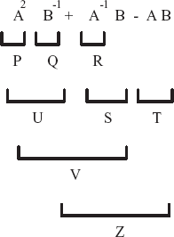
First level grouping:
This is followed by the second-level grouping:
Then, the third-level grouping:
V =U + S.
And the fourth-level grouping:
Z = V − T.
The diagram in Figure 2.2 is a tree with the root at Z. Each grouping described above is represented as a call to the corresponding function in main(). Supposing g is the object linked in main() to those functions, the C++ solution to the expression Z = A2B−1 + A−1B − AB is given as follows:
g.ReadData(A,B);
g.MatMultiply(P,A,A);
g.MatInverse(Q,B);
g.MatInverse(R,A);
g.MatMultiply(U,P,Q);
g.MatMultiply(S,R,B);
g.MatMultiply(T,A,B);
g.MatAdd(1,V,U,S);
g.MatAdd(0,Z,V,T);
In the above solution, MatAdd(), MatMultiply(), and MatInverse() are the matrix addition, multiplication, and inverse, respectively. Prior to its implementation, data for the matrices are read and passed into main() through ReadData(). In this case, data for the matrices A and B are received from this function. The values for A become an input for MatMultiply (P,A,A), which performs the multiplication A*A and stores the result in a new matrix P. Similarly, MatInverse(Q,B) receives data for matrix B, computes its inverse of B, and stores the result into a new matrix Q. The function MatAdd(1,V,U,S) adds the matrices U and S and then stores the result into V. The Boolean parameter 1 here means addition, or V=U+S; with 0 the function performs substraction, or V=U-S.
The above code is demonstrated in its complete form in Code2F.cpp with A and B matrices defined in a file called Code2F.in, as follows:
Code2F.cpp: computing Z = A2B− 1 + A− 1B − AB.
#include <fstream.h>
#include <iostream.h>
#define N 3

class MatAlgebra
{
public:
      MatAlgebra() { }
      ~MatAlgebra() { }
      void ReadData(double **,double **);
      void MatAdd(bool,double **,double **,double **);
      void MatInverse(double **,double **);
      void MatMultiply(double **,double**,double **);
};

void MatAlgebra::ReadData(double **a,double **b)
{
      int i,j;
      ifstream InFile("Code2F.in");
      for (i=1;i<=N;i++)
            for (j=1;j<=N;j++)
                  InFile >> a[i][j];
      for (i=1;i<=N;i++)
            for (j=1;j<=N;j++)
                  InFile >> b[i][j];
      InFile.close();
}

void MatAlgebra::MatAdd(bool flag,double **c,double **a,
      double **b)
{
      int i,j,k;
      for (i=1;i<=N;i++)
            for (j=1;j<=N;j++)
                  c[i][j]=((flag)?a[i][j]+b[i][j]:
                          a[i][j]-b[i][j]);
}
void MatAlgebra::MatMultiply(double **c,double **a,double **b)
{
      int i,j,k;
      for (i=1;i<=N;i++)
            for (j=1;j<=N;j++)
{
c[i][j]=0;
for (k=1;k<=N;k++)
c[i][j] += a[i][k]*b[k][j];
}
}
void MatAlgebra::MatInverse(double **x,double **a)
{
int i,j,k;
double Sum,m;
double **b, **q;
b=new double *[N+1];
q=new double *[N+1];
for (i=0; i<=N; i++)
{
b[i]=new double [N+1];
q[i]=new double [N+1];
}
for (i=1;i<=N;i++)
for (j=1;j<=N;j++)
{
b[i][j]=0;
q[i][j]=a[i][j];
if (i==j)
b[i][j]=1;
}
// Perform row operations
for (k=1;k<=N-1;k++)
for (i=k+1;i<=N;i++)
{
m=q[i][k]/q[k][k];
for (j=1;j<=N;j++)
{
q[i][j]-=m*q[k][j];
b[i][j]-=m*b[k][j];
}
}
// Perform back subscriptstitution
for (i=N;i>=1;i--)
for (j=1;j<=N;j++)
{
Sum=0;
x[i][j]=0;for (k=i+1;k<=N;k++)
Sum += q[i][k]*x[k][j];
x[i][j]=(b[i][j]-Sum)/q[i][i];
}
for (i=0;i<=N;i++)
delete b[i], q[i];
delete b, q;
}
void main()
{
int i,j;
double **A,**B;
double **P,**Q,**R,**S,**T,**U,**V,**Z;
MatAlgebra g;
A=new double *[N+1];
B=new double *[N+1];
P=new double *[N+1];
Q=new double *[N+1];
R=new double *[N+1];
S=new double *[N+1];
T=new double *[N+1];
U=new double *[N+1];
V=new double *[N+1];
Z=new double *[N+1];
for (i=0;i<=N;i++)
{
A[i]=new double [N+1];
B[i]=new double [N+1];
P[i]=new double [N+1];
Q[i]=new double [N+1];
R[i]=new double [N+1];
S[i]=new double [N+1];
T[i]=new double [N+1];
U[i]=new double [N+1];
V[i]=new double [N+1];
Z[i]=new double [N+1];
}
cout.setf(ios::fixed);
cout.precision(12);
g.ReadData(A,B);
g.MatMultiply(P,A,A);
g.MatInverse(Q,B);
g.MatInverse(R,A);
g.MatMultiply(U,P,Q);g.MatMultiply(S,R,B);
g.MatMultiply(T,A,B);
g.MatAdd(1,V,U,S);
g.MatAdd(0,Z,V,T);
for (i=1;i<=N;i++)
{
for (j=1;j<=N;j++)
cout << Z[i][j] << " ";
cout << endl;
}
for (i=0;i<=N;i++)
delete A[i],B[i],P[i],Q[i],R[i],S[i],T[i],U[i],V[i],
Z[i];
delete A,B,P,Q,R,S,T,U,V,Z;
}Not all numbers in existence are real. There are also cases in which a number exists from an imagination based on some undefined entity. Complex number is a number representation based on the imaginary definition of
This definition implies i2 = − 1, which is not possible in the real world. However, the existence of complex numbers cannot be denied as they provide a powerful foundation to several problems in mathematical modeling.
Complex numbers play an important role in numerical computations. For example, in one area of mathematics called conformal mapping, complex numbers are used to map one geometrical shape from a complex plane to another complex plane in such a way to preserve certain quantities. One such work is the mapping of a circular cylinder to a family of airfoil shapes by considering the pressure and velocity of particles around the cylinder. In another area of study called chaotic theory, complex numbers are used in modeling randomly displaced particles in a fluid that are subject to a motion called Brownian movement.
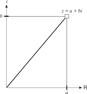
A complex number z has two parts, namely, real and imaginary, defined as follows:
In the above form, a is the real part, whereas b is the imaginary part. A complex number with b = 0 is a real number. Figure 2.3 shows a complex number z = a + bi with respect to the real axis, R and the imaginary axis i, with the origin at z = 0 + 0i = 0.
Complex numbers are not represented directly in their standard form in the computer, because the computer supports integers only in its operations. Therefore, some specialized routines need to be created for manipulating the integers in the computer to enable complex number arithmetic.
In C++, a complex number can be defined using a structure whose contents consist of the real and imaginary parts of the number. For example, the following structure called Complex declares a complex number:
typedef struct
{
      double r;     // real part
      double i;     // imaginary part
}
   Complex;
Using the above structure, a complex number z can be created as an object through the declaration
Complex z;
It follows that z.r represents the real part of z (which is a) and z.i represents the imaginary part of z (which is b), or
z.r =a, and z.i =b.
Arithmetic on complex numbers obeys the same set of rules in mathematics as that of the real numbers. Basically, the operations involve addition, substraction, multiplication, and division. We discuss the development of functions for each of the algebraic tools using a single class called ComAlgebra.
The addition of two complex numbers is carried out by adding their real part and imaginary part separately. The same rule also applies to substraction. Suppose z1 = a1 + b1i and z2 = a2 + b2i are two complex numbers. Then their sum is
Similarly, substraction is carried out as follows:
In C++, addition between two complex numbers u and v is performed using the function Add() to produce w, as follows:
Complex ComAlgebra::Add(Complex u,Complex v)
{
      Complex w;
      w.r = u.r + v.r;
      w.i = u.i + v.i;
      return(w);
}
substraction is very much similar to addition, using the function substract(), as follows:
Complex ComAlgebra::subscripttract(Complex u,Complex v)
{
      Complex w;
      w.r = u.r - v.r;
      w.i = u.i - v.i;
      return(w);
}The multiplication of two complex numbers works in a similar manner as the dot-product between two vectors where the product of the real parts adds to the product of the imaginary parts. For two complex numbers z1 = a1 + b1i and z2 = a2 + b2i, their product is

Multiplication between two numbers, u and v, to produce w is demonstrated using the function Multiply(), as follows:
Complex ComAlgebra::Multiply (Complex u, Complex v)
{
     Complex w;
     w.r = u.r*v.r - u.i*v.i;
     w.i = u.r*v.i + v.r*u.i;
     return(w);
}The conjugate of a complex number z = a + bi is
Complex ComAlgebra::Conjugate(Complex u)
{
      Complex w;
      w.r = u.r;
      w.i = -u.i;
      return(w);
}When a complex number z1 = a1 + b1i is divided by another complex number z2 = a2 + b2i, the result is also a complex number. This calculation is shown as

A function called Divide() shows the division of two complex numbers, u on v, to produce another complex number, w, as follows:
Complex ComAlgebra::Divide(Complex u, Complex v)
{
      Complex c, w, s;
      double denominator;
      c = Conjugate(v);
      s = Multiply (u, c);
      denominator = v.r*v.r + v.i*v.i+ 1.2e-60; // to prevent
                                                   division
                                                   by zero
      w.r = s.r/denominator;
      w.i = s.i/denominator;
      return(w);
}
A variable called denominator in the above code segment has its value added with a very small number 1.2e-60, or 1.2 × 10−60. The addition does not change the result significantly, and it is necessary in order to prevent the value from becoming zero, hence, avoiding the division by zero problem.
The inverse z−1 of a complex number z = a + bi is computed as follows:

The corresponding C++ code using the function Inverse() for computing the inverse of u is shown as follows:
Complex ComAlgebra::Inverse(Complex u)
{
      Complex w,v;
      v.r = 1.0;
      v.i = 0.0;
w = Divide(v,u);
return(w);
}An algebraic arithmetic involving complex numbers is easily performed using the basic operations discussed above: addition, substraction, multiplication, division, conjugate, and inverse. The strategy is to have a function for each operation so that the whole process becomes structured and modular. As demonstrated earlier in the case of matrix operation, an algebraic operation on complex numbers should be based on a good programming principle. To achieve this objective, the operation must maximize the use of local variables, encourage data passing between functions, and encourage object-oriented methodology.
We illustrate complex number algebra using an example in evaluating the expression
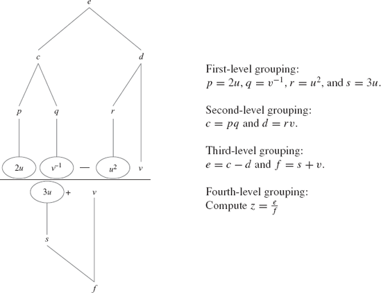
The priority tree in Figure 2.4 is a structured approach for solving the expression
Complex u,v,z,k; Complex p,q,r,s,c,d,e,f; ComAlgebra Compute; k.r=2; k.i=0; p=Compute.Multiply(k,u); q=Compute.Inverse(v); r=Compute.Multiply(u,u); k.r=3; k.i=0; s=Compute.Multiply(k,u); c=Compute.Multiply(p,q); d=Compute.Multiply(r,v); e=Compute.subscripttract(c,d); f=Compute.Add(s,v); z=Compute.Divide(e,f);
Code2G.cpp shows the full program for the algebraic operation in solving the expression
Code2G.cpp: complex number algebra for solving
#include <iostream.h>
#include <math.h>
typedef struct
{
double r; // real part
double i; // imaginary part
} Complex;
class ComAlgebra
{
public:
ComAlgebra();
Complex Add(Complex,Complex);
Complex subscripttract(Complex,Complex);
Complex Conjugate(Complex);
Complex Multiply(Complex,Complex);
Complex Divide(Complex,Complex);
Complex Inverse(Complex);
double Magnitude(Complex);
double Angle(Complex);
};ComAlgebra::ComAlgebra()
{}
Complex ComAlgebra::Add(Complex u,Complex v)
{
Complex w;
w.r = u.r + v.r;
w.i = u.i + v.i;
return(w);
}
Complex ComAlgebra::subscripttract(Complex u,Complex v)
{
Complex w;
w.r = u.r - v.r;
w.i = u.i - v.i;
return(w);
}
Complex ComAlgebra::Conjugate(Complex u)
{
Complex w;
w.r = u.r;
w.i = -u.i;
return(w);
}
Complex ComAlgebra::Multiply (Complex u, Complex v)
{
Complex w;
w.r = u.r*v.r - u.i*v.i;
w.i = u.r*v.i + v.r*u.i;
return(w);
}
Complex ComAlgebra::Divide(Complex u, Complex v)
{
Complex c, w, s;
double denominator;
c = Conjugate(v);
s = Multiply (u, c);
denominator = v.r*v.r +v.i*v.i+ 1.2e-60; //to prevent
division
by zero
w.r = s.r/denominator;w.i = s.i/denominator;
return(w);
}
Complex ComAlgebra::Inverse(Complex u)
{
Complex w,v;
v.r = 1.0;
v.i = 0.0;
w = Divide(v,u);
      return(w);
}
void main()
{
Complex u,v,z,k;
Complex p,q,r,s,c,d,e,f;
ComAlgebra Compute;
u.r=−4; u.i=7;
v.r=6; v.i=3;
k.r=2; k.i=0;
p=Compute.Multiply(k,u);
q=Compute.Inverse(v);
r=Compute.Multiply(u,u);
k.r=3; k.i=0;
s=Compute.Multiply(k,u);
c=Compute.Multiply(p,q);
d=Compute.Multiply(r,v);
e=Compute.subscripttract(c,d);
f=Compute.Add(s,v);
z=Compute.Divide(e,f);
cout << "z = " << z.r << " + "<< z.i << "i" << endl;
}One important feature in numbers is their order based on the values they carry. For example, 3 has a lower value than 7; therefore, 3 should be placed before 7. Arranging numbers in order according to their values helps in making the data more readable and organized. Besides, ordered data contribute toward an efficient searching mechanism and for use in their analysis. The main application involving number sorting can be found in the database management system.
Data can be sorted in the order from lowest to highest, or highest to lowest, based on their numeric or alphabetic values. An integer or double variable is ordered according its numeric value, whereas a string is sorted based on its alphabetical value.
Number sorting is a data structure problem that may require high computational time in its implementation. Number sorting helps in searching for a particular record based on its order.
The code below performs sorting with k steps with a complexity of O(N2), where at each step the numbers w[i] with w[i+1] are compared. If w[i] has a value greater than w[i+1], then the two values are swapped, using tmp as the temporary variable to hold the values before swapping.
for (int k=1;k<=N;k++)
      for (i=1;i<=N-1;i++)
      if (w[i]>w[i+1])     // swap for low to high
      {
            tmp=w[i];
            w[i]=w[i+1];
            w[i+1]=tmp;
       }
Example 2.5. Sort the numbers in the list given by 60, 74, 43, 57 and 45 in ascending order.
Solution. Applying the sorting algorithm above with k = 1:

Continue with k = 2:

Next iteration with k= 3:

The numbers have been fully sorted after k = 3. The final order from the given list is 43, 45, 57, 60, and 74.
Code2H.cpp shows the full C++ program for the sorting problem using random numbers as the input.
Code2H.cpp: sorting numbers
#include <iostream.h>
#include <stdlib.h>
#include <time.h>
#define N 8

void main()
{
      int *v,*w,tmp;
      v = new int [N+1];
      w = new int [N+1];

      time t seed=time(NULL);
      srand((unsigned)seed);

      for (int i=1;i<=N;i++)
      {
           v[i]=1+rand()%100;         // random numbers from 1
                                         to 100
           w[i]=v[i];
      }
      for (int k=1;k<=N;k++)
            for (i=1;i<=N-1;i++)
                 if (w[i]>w[i+1])     // swap for low to high
                 {
                       tmp=w[i];
                       w[i]=w[i+1];
                       w[i+1]=tmp;
                 }
      cout << "the unsorted random numbers v[i] are:" << endl;
for (i=1;i<=N;i++)
cout << v[i] << " ";
cout << endl << "sorted from lowest to highest w[i]:"
<< endl;
for (i=1;i<=N;i++)
cout << w[i] << " ";
cout << endl;
}This chapter outlines the importance of good programming strategies for handling several mathematical-intensive operations involving massive data. The strategies include exploring the resources in the computer to the maximum in order to optimize the operations. This chapter highlights some important programming strategies such as breaking down the program into modules, allocating memory dynamically to arrays, maximizing the use of local variables, and encouraging data passing between functions. It is important to consider these issues seriously in designing the solution as a typical scientific problem often causes the computer to perform below its capability. In some cases, the computer performance is adversely affected through poor management of memory and improper techniques that originate from the spaghetti type of coding.
The main issue regarding scientific computing that affects the computer performance is the handling of arrays. A typical array in an application represents a matrix that often occupies a large amount of computer memory. A good strategy is to allocate memory dynamically to these arrays. Besides memory management, an array is also subject to its mathematical properties and behavior. Any operation involving arrays must be carefully executed by considering their mathematic properties in all steps of the operation. For example, if a given matrix is singular, then it is not possible to find its inverse as the computation will only lead to some bad results.
Data passing is an important issue that contributes toward a structured and modular program design. A good contribution can be seen from the feature in data passing, which encourages the arrays and variables to be declared local, and their values can be shared by another function through this mechanism. This is illustrated through a discussion on how a complex expression involving arrays and vectors can be solved easily through a modular technique that advocates data passing.
We discuss row operations, which is an important technique for reducing a matrix into its simpler form. Row operations involve some massive and tedious calculations that contribute to problems such as finding the determinant of a matrix, reducing a matrix to its triangular form, and finding the inverse of a matrix. Another core application involving row operations is in solving a system of linear equations, and this topic will be discussed thoroughly in the next chapter.
We also explore some mathematical problems involving complex numbers and number sorting. By default, complex numbers are not supported in the computer. But, it is possible to perform operations involving complex numbers by treating the numbers as members of a structure. We show how a difficult mathematical expression involving complex numbers can be solved easily using a modular programming approach.
Number sorting is the extra tool that is included in this chapter. The topic itself falls under the category of data structure, which is not in the scope of our discussion. However, the problem appears quite often in various mathematical and engineering problems. In this chapter, we show how number sorting is performed with programming as its tool.
Code2Cproject computes the upper triangular matrix U from any square matrix A. Write a new program to reduce A into a lower triangular matrix L, as defined in Equation (2.10).An extension to the
Code2Cproject is the decomposition of a square matrix A into the product of its upper and lower triangular matrices, or A = LU. Write a new program to do this.Code2F.cppillustrates a modular approach for solving an algebraic operation involving matrices where the matrices are square and have fixed sizes. Design a C++ program to compute Z = A2B− 1 + A− 1B − AB for matrices A and B that have flexible sizes. The program must provide a check on the dimension and status of each matrix according to the fundamental mathematical properties in order to allow operations such as multiplication and computing the inverse.Modify
Code2F.cppfor solving the following problems:Z = (A + 3B)−1.
Z = A−1B2 + 3A2B−1.
Z = (AB)2 − 3(AB)−1.
An orthogonal matrix is the matrix A = [aij] for i = 1, 2,..., M, and j = 1,2,..., N, where

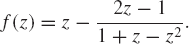
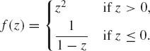
A function f(z) of a complex number z is defined as the mapping from z to f(z) in such a way f(z) is unique. Write a standard C++ program for the following functions:
f(z) = 1 − z.
f(z) = 3 − 2z + 2z2 − z3.