10.1 Bayesian importance sampling

Importance sampling was first mentioned towards the start of Section 9.1. We said then that it is useful when we want to find a parameter θ which is defined as the expectation of a function f(x) with respect to a density q(x) but we cannot easily generate random variables with that density although we can generate variates xi with a density p(x) which is such that p(x) roughly approximates |f(x)|q(x) over the range of integration. Then

The function p(x) is called an importance function. In the words of Wikipedia, ‘Importance sampling is a variance reduction technique that can be used in the Monte Carlo method. The idea behind importance sampling is that certain values of the input random variables in a simulation have more impact on the parameter being estimated than others. If these ‘important’ values are emphasized by sampling more frequently, then the estimator variance can be reduced.’

A case where this technique is easily seen to be valuable occurs in evaluating tail areas of the normal density function (although this function is, of course, well-enough tabulated for it to be unnecessary in this case). If, for example, we wanted to find the probability that a standard normal variate was greater than 4, so that

a naïve Monte Carlo method would be to find the proportion of values of such a variate in a large sample that turned out to be greater than 4. However, even with a sample as large as n=10 000 000 a trial found just 299 such values, implying that the required integral came to 0.000 030 0, whereas a reference to tables shows that the correct value of θ is 0.000 031 67, which is, therefore, underestimated by 5%. In fact, the number we observe will have a binomial distribution and our estimate will have a standard deviation of .

We can improve on this slightly by noting that and therefore the fact that in the same trial 619 values were found to exceed 4 in absolute value leads to an estimate of 0.000 030 95, this time an underestimate by about 2%. This time the standard deviation can easily be shown to be . There are various other methods by which slight improvements can be made (see Ripley, 1987, Section 5.1).

A considerably improved estimate can be obtained by importance sampling with p(x) being the density function of an exponential distribution E(1) of mean 1 (see Appendix A.4) truncated to the range so that

It is easily seen that we can generate a random sample from this density by simply generating values from the usual exponential distribution E(1) of mean 1 and adding 4 to these values. By using this truncated distribution, we avoid needing to generate values which will never be used. We can take then an importance sampling estimator

Using this method, a sample of size only 1000 resulted in an estimate of 0.000 031 5 to three decimal places, which is within 1% of the correct value.

With any importance sampler each observed value x has density p(x) and so w(x)=f(x)q(x)/p(x) has mean

and variance

If for all x and we take

then w(x) is constant and so has variance 0 which is necessarily a minimum. This choice, however, is impossible because to make it we would need to know the value of θ, which is what we are trying to find. Nevertheless, if fq/p is roughly constant then we will obtain satisfactory results. Very poor results occur when fq/p is small with a high probability but can be very large with a low probability, as, for example, when fq has very wide tails compared with p.

For a more complicated example, suppose has a gamma density

(see Section A.4). Then there is a family of conjugate priors of the form

where and are hyperparameters, since the posterior is then equal to

(we write q rather than p in accordance with our notation for importance sampling). This does not come from any of the well-known distributions and the constant of proportionality is unknown, although it can be approximated by normal or gamma densities. In Figure 10.1, we show the unnormalized density when and . It appears symmetric about a value near 1.5 with most of the values between 0.75 and 2.25, so it seems reasonable to use as an importance function an approximation such as N(1.5, 0.75) or, since it is asymmetric, a gamma density with the same mean and variance, so a G(4, 0.375) distribution, and these two are also illustrated in the figure. There is a discrepancy in scale because the constant of proportionality of the density we are interested in is unknown.

Figure 10.1 The conjugate gamma distribution.

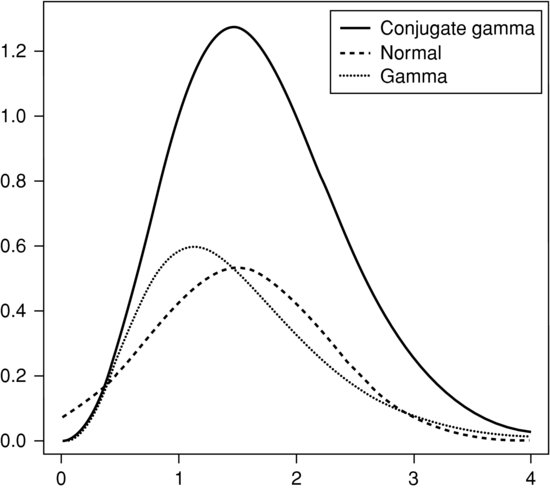
While in the middle of the range either of these distributions fits reasonably well, the gamma approximation is considerably better in the tails. We can begin by finding the constant of proportionality using the importance sampling formula with f(x)=1, and p(x) taken as a gamma density with and . Use of this method with a sample size of 10 000 resulted in a value for the constant of 2.264 where the true value is approximately 2.267. We can use the same sample to find a value of the mean, this time taking f(x)=x/k and finding a value of 1.694 where the true value is 1.699 (we would have taken a different importance function if we were concerned only with this integral, but when we want results for both f(x)=1 and f(x)=x/k it saves time to use the same sample). In the same way we can obtain a value of 0.529 for the variance where the true value is 0.529.

10.1.1 Importance sampling to find HDRs

It has been pointed out (see Chen and Shao, 1998) that we can use importance sampling to find HDRs. As we noted in Section 2.6, an HDR is an interval which is (for a given probability level) as short as possible. This being so, all we need to do is to take the sample generated by importance sampling, sort it and note that for any desired value α, if the sorted vales are and , then any interval of the form (yj, yj+k) will give an interval with an estimated posterior probability of , so for an HDR we merely need to find the shortest such interval. It may help to consider the following segment of code:

alpha < - 0.1
le <- (1-alpha)*n
lo <- 1:(n-le)
hi <- (le+1):n
y <- sort(samp)
r <- y[hi]-y[lo]
rm <- min(r)
lom <- min(lo[r==rm])
him <- min(hi[r==rm])
abline(v=y[lom])
abline(v=y[him])

10.1.2 Sampling importance re-sampling

Another technique sometimes employed is sampling importance re-sampling (SIR). This provides a method for generating samples from a probability distribution which is hard to handle and for which the constant of proportionality may be unknown. We suppose that the (unnormalized) density in question is q(x). What we do is to generate a sample of size n from a distribution with density p(x) which is easier to handle and is in some sense close to the distribution we are interested in. We then find the values of

and then normalize these to find

We then take a sample of the same size size n without replacement from the values with probabilities to obtain a new sample . This operation is easily carried out in by

x <- random sample of size n from density p
w <- q(x)/p(x)
pi <- w/sum(w)
samp <- sample(x,size=n,prob=pi,replace=T)

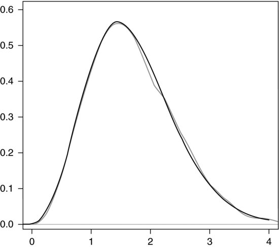
The success of this method is illustrated in Figure 10.2, where the normalized conjugate density discussed earlier is compared with the smoothed density function found from such a random sample constructed in this way starting from the gamma approximation.

Figure 10.2 Approximation to the conjugate gamma distribution.

We have used sampling with replacement as recommended by Albert (2009, Section 5.10), although Gelman et al. (2004, Section 10.5) prefer sampling without replacement, claiming that ‘in a bad case, with a few very large values and many small values [s]ampling with replacement will pick the same few values … again and again; in contrast, sampling without replacement yields a more desirable intermediate approximation’. Nevertheless, at least in some cases such as the one discussed here, substituting replace=F results in a much poorer fit.

We can, of course, use the sample thus obtained to estimate the mean, this time as 1.689, and the variance, this time as 0.531. Further, we can use these values to estimate the median as 1.616 where the true value is 1.622.

10.1.3 Multidimensional applications

The SIR algorithm is most commonly applied in situations when we are trying to find the properties of the posterior distribution of a multidimensional unknown parameter . Quite often, it turns out that a convenient choice of an approximating density p from which to generate a random sample is the multivariate t distribution. Since the multivariate t distribution has been avoided in this book, we shall not discuss this approach further; for more details about it see Albert (2009, Section 5.10).