1.1 Probability and Bayes’ Theorem

1.1.1 Notation

The notation will be kept simple as possible, but it is useful to express statements about probability in the language of set theory. You probably know most of the symbols undermentioned, but if you do not you will find it easy enough to get the hang of this useful shorthand. We consider sets of elements and we use the word ‘iff’ to mean ‘if and only if’. Then we write

Let (An) be a sequence of sets. Then

We sometimes need a notation for intervals on the real line, namely

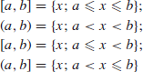
where a and b are real numbers or or .

1.1.2 Axioms for probability

In the study of probability and statistics, we refer to as complete a description of the situation as we need in a particular context as an elementary event.

Thus, if we are concerned with the tossing of a red die and a blue die, then a typical elementary event is ‘red three, blue five’, or if we are concerned with the numbers of Labour and Conservative MPs in the next parliament, a typical elementary event is ‘Labour 350, Conservative 250’. Often, however, we want to talk about one aspect of the situation. Thus, in the case of the first example, we might be interested in whether or not we get a red three, which possibility includes ‘red three, blue one’, ‘red three, blue two’, etc. Similarly, in the other example, we could be interested in whether there is a Labour majority of at least 100, which can also be analyzed into elementary events. With this in mind, an event is defined as a set of elementary events (this has the slightly curious consequence that, if you are very pedantic, an elementary event is not an event since it is an element rather than a set). We find it useful to say that one event E implies another event F if E is contained in F. Sometimes it is useful to generalize this by saying that, given H, E implies F if EH is contained in F. For example, given a red three has been thrown, throwing a blue three implies throwing an even total.

Note that the definition of an elementary event depends on the context. If we were never going to consider the blue die, then we could perfectly well treat events such as ‘red three’ as elementary events. In a particular context, the elementary events in terms of which it is sensible to work are usually clear enough.

Events are referred to above as possible future occurrences, but they can also describe present circumstances, known or unknown. Indeed, the relationship which probability attempts to describe is one between what you currently know and something else about which you are uncertain, both of them being referred to as events. In other words, for at least some pairs of events E and H there is a number defined which is called the probability of the event E given the hypothesis H. I might, for example, talk of the probability of the event E that I throw a red three given the hypothesis H that I have rolled two fair dice once, or the probability of the event E of a Labour majority of at least 100 given the hypothesis H which consists of my knowledge of the political situation to date. Note that in this context, the term ‘hypothesis’ can be applied to a large class of events, although later on we will find that in statistical arguments, we are usually concerned with hypotheses which are more like the hypotheses in the ordinary meaning of the word.

Various attempts have been made to define the notion of probability. Many early writers claimed that was m/n where there were n symmetrical and so equally likely possibilities given H of which m resulted in the occurrence of E. Others have argued that should be taken as the long run frequency with which E happens when H holds. These notions can help your intuition in some cases, but I think they are impossible to turn into precise, rigourous definitions. The difficulty with the first lies in finding genuinely ‘symmetrical’ possibilities – for example, real dice are only approximately symmetrical. In any case, there is a danger of circularity in the definitions of symmetry and probability. The difficulty with the second is that we never know how long we have to go on trying before we are within, say, 1% of the true value of the probability. Of course, we may be able to give a value for the number of trials we need to be within 1% of the true value with, say, probability 0.99, but this is leading to another vicious circle of definitions. Another difficulty is that sometimes we talk of the probability of events (e.g. nuclear war in the next 5 years) about which it is hard to believe in a large numbers of trials, some resulting in ‘success’ and some in ‘failure’. A good, brief discussion is to be found in Nagel (1939) and a fuller, more up-to-date one in Chatterjee (2003).

It seems to me, and to an increasing number of statisticians, that the only satisfactory way of thinking of is as a measure of my degree of belief in E given that I know that H is true. It seems reasonable that this measure should abide by the following axioms:

P1		for all E, H.
P2		= 1  for all H.
P3		when .
P4

By taking in P3 and using P1 and P2, it easily follows that

so that is always between 0 and 1. Also by taking in P3 it follows that

Now intuitive notions about probability always seem to agree that it should be a quantity between 0 and 1 which falls to 0 when we talk of the probability of something we are certain will not happen and rises to 1 when we are certain it will happen (and we are certain that H is true given H is true). Further, the additive property in P3 seems highly reasonable – we would, for example, expect the probability that the red die lands three or four should be the sum of the probability that it lands three and the probability that it lands four.

Axiom P4 may seem less familiar. It is sometimes written as

although, of course, this form cannot be used if the denominator (and hence the numerator) on the right-hand side vanishes. To see that it is a reasonable thing to assume, consider the following data on criminality among the twin brothers or sisters of criminals [quoted in his famous book by Fisher (1925b)]. The twins were classified according as they had a criminal conviction (C) or not (N) and according as they were monozygotic (M) (which is more or less the same as identical – we will return to this in Section 1.2) or dizygotic (D), resulting in the following table:

If we denote by H the knowledge that an individual has been picked at random from this population, then it seems reasonable to say that

If on the other hand, we consider an individual picked at random from among the twins with a criminal conviction in the population, we see that

and hence

so that P4 holds in this case. It is easy to see that this relationship does not depend on the particular numbers that happen to appear in the data.

In many ways, the argument in the preceding paragraph is related to derivations of probabilities from symmetry considerations, so perhaps it should be stressed that while in certain circumstances we may believe in symmetries or in equally probable cases, we cannot base a general definition of probability on such arguments.

It is convenient to use a stronger form of axiom P3 in many contexts, namely,

whenever the (En) are exclusive events given H. There is no doubt of the mathematical simplifications that result from this assumption, but we are supposed to be modelling our degrees of belief and it is questionable whether these have to obey this form of the axiom. Indeed, one of the greatest advocates of Bayesian theory, Bruno de Finetti, was strongly against the use of P3*. His views can be found in de Finetti (1972, Section 5.32) or in de Finetti (1974–1975, Section 3.11.3).

There is certainly some arbitrariness about P3*, which is sometimes referred to as an assumption of σ-additivity, in that it allows additivity over some but not all infinite collections of events (technically over countable but not over uncountable collections). However, it is impossible in a lot of contexts to allow additivity over any (arbitrary) collection of events. Thus, if we want a model for picking a point ‘completely at random’ from the unit interval

it seems reasonable that the probability that the point picked is in any particular sub-interval of the unit interval should equal the length of that sub-interval. However, this clearly implies that the probability of picking any one particular x is zero (since any such x belongs to intervals of arbitrarily small lengths). But the probability that some x is picked is unity, and it is impossible to get one by adding a lot of zeroes.

Mainly because of its mathematical convenience, we shall assume P3* while being aware of the problems.

1.1.3 ‘Unconditional’ probability

Strictly speaking, there is, in my view, no such thing as an unconditional probability. However, it often happens that many probability statements are made conditional on everything that is part of an individual’s knowledge at a particular time, and when many statements are to be made conditional on the same event, it makes for cumbersome notation to refer to this same conditioning event every time. There are also cases where we have so much experimental data in circumstances judged to be relevant to a particular situation that there is a fairly general agreement as to the probability of an event. Thus, in tossing a coin, you and I both have experience of tossing similar coins many times and so are likely to believe that ‘heads’ is approximately as likely as not, so that the probability of ‘heads’ is approximately given your knowledge or mine.

In these cases we write

where Ω is the set of possibilities consistent with the sum total of data available to the individual or individuals concerned. We usually consider sets F for which , so that . It easily follows from the axioms that

whenever the (En) are exclusive events (or more properly whenever they are exclusive events given Ω), and

Many books begin by asserting that unconditional probability is an intuitive notion and use the latter formula in the form

to define conditional probability.

1.1.4 Odds

It is sometimes convenient to use a language more familiar to bookmakers to express probabilistic statements. We define the odds on E against F given H as the ratio

or equivalently

A reference to the odds on E against F with no mention of H is to be interpreted as a reference to the odds on E against F given Ω , where Ω is some set of background knowledge as above.

Odds do not usually have properties as simple as probabilities, but sometimes, for example, in connection with Bayesian tests of hypotheses, they are more natural to consider than separate probabilities.

1.1.5 Independence

Two events E and F are said to be independent given H if

From axiom P4, it follows that if this condition is equivalent to

so that if E is independent of F given H then the extra information that F is true does not alter the probability of E from that given H alone, and this gives the best intuitive idea as to what independence means. However, the restriction of this interpretation to the case where makes the original equation slightly more general.

More generally, a sequence (En) of events is said to be pairwise independent given H if

and is said to consist of mutually independent events given H if for every finite subset of them

You should be warned that pairwise independence does not imply mutual independence and that

is not enough to ensure that the finite sequence consists of mutually independent events given H.

Naturally, if no conditioning event is explicitly mentioned, the probabilities concerned are conditional on Ω as defined above.

1.1.6 Some simple consequences of the axioms; Bayes’ Theorem

We have already noted a few consequences of the axioms, but it is useful at this point to note a few more. We first note that it follows simply from P4 and P2 and the fact that HH=H that

and in particular

Next note that if, given H, E implies F, that is and so EFH=EH, then by P4 and the aforementioned equation

From this and the fact that it follows that if, given H, E implies F, then

In particular, if E implies F then

For the rest of this subsection, we can work in terms of ‘unconditional’ probabilities, although the results are easily generalized. Let (Hn) be a sequence of exclusive and exhaustive events, and let E be any event. Then

since by P4 the terms on the right-hand side are , allowing us to deduce the result from P3*. This result is sometimes called the generalized addition law or the law of the extension of the conversation.

The key result in the whole book is Bayes’ Theorem. This is simply deduced as follows. Let (Hn) be a sequence of events. Then by P4

so that provided

This relationship is one of several ways of stating Bayes’ Theorem, and is probably the best way in which to remember it. When we need the constant of proportionality, we can easily see from the above that it is .

It should be clearly understood that there is nothing controversial about Bayes’ Theorem as such. It is frequently used by probabilists and statisticians, whether or not they are Bayesians. The distinctive feature of Bayesian statistics is the application of the theorem in a wider range of circumstances than is usual in classical statistics. In particular, Bayesian statisticians are always willing to talk of the probability of a hypothesis, both unconditionally (its prior probability) and given some evidence (its posterior probability), whereas other statisticians will only talk of the probability of a hypothesis in restricted circumstances.

When (Hn) consists of exclusive and exhaustive events, we can combine the last two results to see that

A final result that we will find useful from time to time is the generalized multiplication law, which runs as follows. If are any events then

provided all the requisite conditional probabilities are defined, which in practice they will be provided . This result is easily proved by repeated application of P4.