8.2 The hierarchical normal model

8.2.1 The model

Suppose that

is a vector of fixed, unknown parameters and that

is a vector of independent observations such that

Of course, the Xi could each be means of a number of observations.

For the moment, we shall suppose that is known, so, after a suitable normalization, we can suppose that .

It is useful to establish some notation for use later on, We shall consider a fixed origin

and we will write

and

for a vector of r elements all equal to unity.

We suppose that on the basis of our knowledge of the Xi we form estimates of the and write

In general, our estimates will not be exactly right and we will adopt a decision theoretic approach as described in Section 7.5 on ‘Bayesian decision theory’. In particular, we shall suppose that by estimating the parameters we suffer a loss

We recall that the risk function is defined as

For our problem the ‘obvious’ estimator (ignoring the hierarchical structure which will be introduced later) is

and indeed since the log-likelihood is

it is the maximum likelihood estimator. It is clearly unbiased.

It is easy to find the risk of this obvious estimator – it is

8.2.2 The Bayesian analysis for known overall mean

To express this situation in terms of a hierarchical model, we need to suppose that the parameters come from some population, and the simplest possibility is to suppose that

in which case it is convenient to take . With the additional structure assumed for the means, the problem has the structure of a situation variously described as a random effects model, Model II or a components of variance model (cf. Eisenhart et al., 1947, or Scheffé, 1959, Section 7.2, n.7). We are, however, primarily interested in the means and not in the variance components and , at least for the moment.

It follows that the posterior distribution of given is

where (writing )

and

(cf. Section 2.2 on ‘Normal Prior and Likelihood’).

To minimize the expectation of the loss over the posterior distribution of , it is clearly necessary to use the Bayes estimator

where

the posterior mean of given (see the subsection of Section 7.5 on ‘Point estimators resulting from quadratic loss’). Further, if we do this, then the value of this posterior expected loss is

It follows that the Bayes risk

(the expectation being taken over values of ) is

We note that if instead we use the maximum likelihood estimator , then the posterior expected loss is increased by an amount

which is always positive, so that

Further, since the unconditional distribution of Xi is evidently , so that , its expectation over repeated sampling (the Bayes risk) is

This is, in fact, obvious since we can also write

where the expectation is over , and since for the maximum likelihood estimator =1 for all , we have

We can thus see that use of the Bayes estimator always diminishes the posterior loss, and that the amount ‘saved’ by its use averages out at λ over repeated sampling.

8.2.3 The empirical Bayes approach

Typically, however, you will not know (or equivalently λ). In such a situation, you can attempt to estimate it from the data. Since the Xi have an unconditional distribution which is , it is clear that S1 is a sufficient statistic for , or equivalently for λ, which is such that or

so that if we define

then using the probability density of a chi-squared distribution (as given in Appendix A)

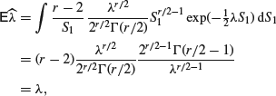
so that is an unbiased estimator of λ.

Now consider the effect of using the empirical Bayes estimator

which results from replacing λ by in the expression for . If we use this, then the value of the posterior expected loss exceeds that incurred by the Bayes rule by an amount

which is always positive, so that

Further, if we write (so that and ), then we see that the expectation of over repeated sampling is

It follows that the Bayes risk resulting from the use of the empirical Bayes estimator is

as opposed to for the Bayes estimator or 1 for the maximum likelihood estimator.