Chapter 6. Deep learning and neural networks

This chapter covers

• Neural network basics
• An introduction to deep learning
• Digit recognition using restricted Boltzmann machines

There is much discussion about deep learning at the moment, and it’s widely seen to be the next big advance in machine learning and artificial intelligence. In this chapter, we’d like to cut through the rhetoric to provide you with the facts. At the end of this chapter, you should understand the basic building block of any deep learning network, the perceptron, and understand how these fit together in a deep network. Neural networks heralded the introduction of the perceptron, so we’ll discuss these before exploring deeper, more expressive networks. These deeper networks come with significant challenges in representation and training, so we need to ensure a good foundational knowledge before leaping in.

Before we do all of this, we’ll discuss the nature of deep learning and the kinds of problems deep learning has been applied to and what makes these successful. This should give you a foundational motivation for deep learning and a frame on which to hang some of the more complicated theoretical concepts later in the chapter. Remember that this is a still a vibrant and active area of research in the community, so I recommend that you keep abreast of the latest advances by following the literature. Startup.ML^[1] and KDNuggets^[2] are just a couple of the resources that can provide you with an up-to-date summary of what’s happening in the community. But I urge you to do your own research and come up with your own conclusions!

¹

Startup.ML, “Deep Learning News,” June 30, 2015, http://news.startup.ml.

²

KDNuggets, “Deep Learning,” www.kdnuggets.com/tag/deep-learning.

6.1. An intuitive approach to deep learning

In order to understand deep learning, let’s choose the application of image recognition; namely, given a picture or a video, how do we build classifiers that will recognize objects? Such an application has potentially wide-reaching applications. With the advent of the quantified self^[3], ^[4] and Google Glass, we could imagine applications that recognize objects visible to the user and provide augmented visuals through their glasses.

³

Gina Neff and Dawn Nafus, The Quantified Self (MIT Press, 2016).

⁴

Deborah Lupton, The Quantified Self (Polity Press, 2016).

Let’s take the example of recognizing a car. Deep learning builds up layers of understanding, with each layer utilizing the previous one. Figure 6.1 shows some of the possible layers of understanding for a deep network trained to recognize cars. Both this example and some of the images that follow have been reproduced from Andrew Ng’s lecture on the subject.^[5]

⁵

Andrew Ng, “Bay Area Vision Meeting: Unsupervised Feature Learning and Deep Learning,” YouTube, March 7, 2011, http://mng.bz/2cR9.

Figure 6.1. Visualizing a deep network for recognizing cars. Some graphical content reproduced from Andrew Ng’s talk on the subject, cited previously. A base training set of pictures is used to create a basis of edges. These edges can be combined to detect parts of cars, and these parts of cars can be combined to detect an object type, which is in this case a car.

At the bottom of figure 6.1, you can see a number of stock images of cars. We’ll consider these our training set. The question is, how do we use deep learning to recognize the similarities between these images: that is, that they all contain a car, possibly without any hand-labeled ground truth? The algorithm isn’t told that the scene contains a car.

As you’ll see, deep learning relies on progressively higher-concept abstractions built directly from lower-level abstractions. In the case of our image-recognition problem, we start out with the smallest element of information in our pictures: the pixel. The entire image set is used to construct a basis of features—think back to chapter 2, where we discussed extracting structure from data—that can be used in composite to detect a slightly higher level of abstraction such as lines and curves. In the next-highest level, these lines are curves that are combined to create parts of cars that have been seen in the training set, and these parts are further combined to create object detectors for a whole car.

There are two important concepts to note here. First, no explicit feature engineering has been performed. If you remember, in the last chapter, we talked about the importance of creating a good representation of your data. We discussed this in the context of click prediction for advertising and noted that experts in the space typically perform this manually. But in this example, unsupervised feature learning has been performed; that is, representations of the data have been learned without any explicit interaction from the user. This may parallel how we as humans may perform recognition—and we’re very good at pattern recognition indeed!

The second important fact to note is that the concept of a car hasn’t been made explicit. Given sufficient variance in the input set of pictures, the highest-level car detectors should do sufficiently well on any car presented. Before we get ahead of ourselves, though, let’s clear up some of the basics around neural networks.

6.2. Neural networks

Neural networks aren’t a new technology by any means and have been around since the 1940s. They’re a biologically inspired concept whereby an output neuron is activated based on the input from several connected input neurons. Neural networks are sometimes known as artificial neural networks, because they achieve artificially a functionality similar to that of a human neuron. Jeubin Huang^[6] provides an introduction to the biology of the human brain. Although many aspects of the functionality of the human brain are still a mystery, we’re able to understand the basic building blocks of operation—but how this gives rise to consciousness is another matter.

⁶

Jeubin Huang, “Overview of Cerebral Function,” Merck Manual, September 1, 2015, http://mng.bz/128W.

Neurons in the brain use a number of dendrites to collect both positive (excitative) and negative (inhibitory) output information from other neurons and encode this electrically, sending it down an axon. This axon splits and reaches hundreds or thousands of dendrites attached to other neurons. A small gap exists between the axon and the input dendrites of the next neuron, and this gap is known as a synapse. Electrical information is converted into chemical output that then excites the dendrite of the next neuron. In this scenario, learning is encoded by the neuron itself. Neurons send messages down their axon only if their overall excitation is large enough.

Figure 6.2 shows the schematic of a human biological neuron and an artificial neuron developed by McCulloch and Pitts, the so-called MCP model.^[7] The artificial neuron is built using a simple summation and threshold value and works as follows. Logic inputs, positive only, are received from the dendrite equivalents, and a weighted summation is performed. If this output exceeds a certain threshold and no inhibitory input is observed, a positive value is emitted. If an inhibitory input is observed, the output is inhibited. This output may then be fed onward to the input of other such neurons through their dendrites’ equivalent inputs. A little thought will reveal that this is—ignoring the inhibitory input—a linear model in n-dimensional space, with linked coefficients, where n is the number of inputs to the neuron. Note that in this case, we assume that all dendrite inputs are from different sources; but in theory, the same source can be attached multiple times if we wish for it to be considered more important. This is equivalent to increasing the weight of that input.

⁷

Warren S. McCulloch and Walter H. Pitts, “A Logical Calculus of the Ideas Immanent in Nervous Activity,” Bulletin of Mathematical Biophysics 5 (1943): 115–33.

Figure 6.2. On the left, we provide a schematic of a human biological neuron. To the right, we show a human-inspired neural network implemented using weighted summation, an inhibitory input, and a threshold.

Figure 6.3 illustrates the behavior of this model for n=1. In this illustration, we use a simple hand-built neuron with a unit weight (w=1). The input to the neuron is allowed to vary from -10 to 10, and the summation of the weighted input values is provided on the y-axis. Choosing a threshold of 0, the neuron will fire if the input is greater than 0 but not otherwise.

Figure 6.3. MCP as a 2-D linear model without inhibitory input. The weights of the model correspond to the coefficients of a linear model. In this case, our neuron supports only a single input, and the weight has been set to 1 for illustration. Given a threshold of 0, all inputs with a value less than or equal to 0 would inhibit the neuron from firing, whereas all inputs with a value greater than 0 would cause the neuron to fire.

6.3. The perceptron

In the previous section, we introduced the MCP neuron. With this basic approach, it turns out that it’s possible to learn and to generalize training data, but in a very limited fashion. But we can do better, and thus the perceptron was born. The perceptron builds on the MCP model in three important ways:^[8], ^[9]

⁸

Frank Rosenblatt, The Perceptron—A Perceiving and Recognizing Automaton (Cornell Aeronautical Laboratory, 1957).

⁹

Rosenblatt, “The Perceptron: A Probabilistic Model for Information Storage and Organization in the Brain,” Psychological Review 65, no. 6 (November 1958): 386–408.

• A threshold bias was added as an input to the summation. This serves several equivalent purposes. First, it allows bias to be captured from the input neurons. Second, it means output thresholds can be standardized around a single value, such as zero, without loss of generality.
• The perceptron allows input weights to be independent and negative. This has two important effects. First, a neuron doesn’t need to be connected to an input multiple times to have a greater impact. Second, any dendrite input can be considered inhibitory (although not completely so) if it has a negative weight.
• The development of the perceptron heralded the development of an algorithm to learn the best weights given a set of input and output data.

Figure 6.4 provides a graphical overview of this new extended model. As before, an intermediate value is created using the weighted summation of the inputs, but we now notice the inclusion of a bias value, w₀. This is learned along with the input weights during the training step; more about this in the following sections. The intermediate value, denoted by a here, is then passed through a threshold function to obtain the final result, y.

Figure 6.4. The perceptron. Inputs x₁ through x_n are received and multiplied by their associated weight, with perceptron bias, w₀, being added in afterward. This output, given by a, is then passed through a threshold function to obtain the output.

6.3.1. Training

Now that you know that a neural network consists of many more basic elements called perceptrons, let’s look at how to train a perceptron in isolation. What does it mean to train a perceptron? Let’s take a more concrete example using the logical AND function. We’ll consider a perceptron of two binary inputs with a binary threshold activation function around 0. How do we learn the weights, such that the output of the perceptron is 1, if and only if the two inputs are both equal to 1? Put another way, can we choose continuous valued weights such that the weighted sum of the inputs is greater than 0 when the two inputs are both 1, with the output being less than 0 otherwise? Let’s formalize this problem. We give x as our vector of binary input values and w as our vector of continuous input weights:

x = (x₁, x₂), w = (w₁, w₂)

Thus, we need to learn weights such that the following restrictions hold true for combinations of binary inputs x₁, x₂:

Unfortunately for us, there are no solutions if we pose the problem like this! There are two options to make this problem tractable. Either we allow the threshold to move, defining it as a value not equal to 0, or we introduce an offset; both are equivalent. We’ll opt for the latter in this text, providing these new vectors:

x = (1, x₁, x₂), w = (w₀, w₁, w₂)

Our existing equalities remain the same. You can now see that with careful weight selection, we can create the AND function. Consider the case where w₁ = 1, w₂ = 1, and w₀ = –1.5. Table 6.1 provides the output from our perceptron and the output from the AND function.

Table 6.1. Comparing the output of our perceptron with the output of the logical AND function, which returns 1 if both inputs are equal to 1. Results provided are for the case where w₁ = 1, w₂ = 1, and w₀ = –1.5.

x1	x2	w0	Weighted sum	Sign of weighted sum	x1 AND x2
1	0	–1.5	–0.5	Negative	0
0	1	–1.5	–0.5	Negative	0
0	0	–1.5	–1.5	Negative	0
1	1	–1.5	0.5	Positive	1

Now that we understand that it’s indeed possible to represent a logical AND using a perceptron, we must develop a systematic way to learn our weights in a supervised manner. Put another way, given a dataset consisting of inputs and outputs, related linearly in this case, how do we learn the weights of our perceptron? We can achieve this using the perceptron algorithm developed by Rosenblatt.^[10], ^[11] The following listing presents the pseudo code used for learning.

¹⁰

Rosenblatt, “The Perceptron: A Probabilistic Model for Information Storage and Organization in the Brain.”

¹¹

Rosenblatt, Principles of Neurodynamics; Perceptrons and the Theory of Brain Mechanisms (Spartan Books, 1962).

Listing 6.1. The perceptron learning algorithm

Initialize w to contain random small numbers

For each item in training set:
    Calculate the current output of the perceptron for the item.
    For each weight, update, depending upon output correctness.

So far, so good. Looks easy, right? We start with some small random values for our weights and then iterate over our data points and update the weights depending on the correctness of our perceptron. In fact, we update the weights only if we get the output wrong; otherwise, we leave the weights alone. Furthermore, we update the weights such that they become more like their input vectors in magnitude but with the corresponding sign of the output value. Let’s write this down more formally, as shown in the next listing.

Listing 6.2. The perceptron learning algorithm (2)

Provided the input data is linearly separable, such an algorithm is guaranteed to converge to a solution.^[12]

¹²

Brian Ripley, Pattern Recognition and Neural Networks (Cambridge University Press, 1996).

6.3.2. Training a perceptron in scikit-learn

Previously, we presented the simplest form of a neural network, the perceptron; we also discussed how this algorithm is trained. Let’s now move to scikit-learn and explore how we can train a perceptron using some data. The next listing provides the code to perform the necessary imports and create a NumPy array of data points.

Listing 6.3. Creating data for perceptron learning

In listing 6.3, we perform the necessary imports for the single-perceptron example and create a very small dataset with only four data points. This dataset is contained within a NumPy array called data. Each data point is assigned to either the class 0 or the class 1, with these classes being stored within the target array. Figure 6.5 provides a graphical overview of this data.

Figure 6.5. Graphical overview of the data for a single perceptron. Data with class label 1 is represented by a round dot, whereas data with class label 0 is represented by a star. It’s the aim of the perceptron to separate these points.

In the figure, the only data point with a positive class (with a label of 1) is found at coordinate (1,1) and represented by a round dot. All other data points are associated with the negative class. The following listing provides the sample code to train our simple perceptron and to return the coefficients (w₁,w₂ relating to x₁ and x₂, respectively) along with the bias w₀.

Listing 6.4. Training a single perceptron

The output is similar to the following:

Perceptron(alpha=0.0001, class_weight=None, eta0=1.0, fit_intercept=True,
      n_iter=100, n_jobs=1, penalty=None, random_state=0, shuffle=False,
      verbose=0, warm_start=False)
Coefficients: [[ 3.  2.]] ,Intercept: [-4.]

The first line provides the parameters under which the perceptron was trained; the second provides the output weights and bias of the perceptron. Don’t worry if the coefficients and the intercept are slightly different when you run this. There are many solutions to this problem, and the learning algorithm can return any of them. For a greater understanding of the parameters, I encourage you to read the associated scikit-learn documentation.^[13]

¹³

scikit-learn, “Perceptron,” http://mng.bz/U20J.

6.3.3. A geometric interpretation of the perceptron for two inputs

In our example, we’ve successfully trained a single perceptron and returned the weights and bias of the final perceptron. Great! But how do we interpret these weights in an intuitive way? Luckily, this is easily possible in 2-D space, and we can extend this intuition into higher-dimensional spaces also.

Let’s consider the perceptron for two input values only. From figure 6.4 we have

y = w₀ + w₁x₁ + w₂x₂

This should look familiar to you as the equation of a plane (three dimensions) in x₁, x₂, and y. If they’re not equivalent, this plane intersects with the viewing plane of figure 6.5, and you’re left with a line. When viewed from the point of reference of figure 6.5, points to one side of the line correspond to values of x · w > 0, whereas points on the other side of the line correspond to values of x · w < 0. Points on the line correspond to x · w = 0. Let’s take the concrete example from earlier and visualize this. Using the coefficients just learned, we have the equation of a plane given by

y = – 4 + 3x₁ + 2x₂

The value of y is at 90 degrees to the (x₁,x₂) plane and thus can be thought of as along a line following the eyes of the viewer, straight through the viewing plane. The value of y on the viewing plane is given by 0, so we can find the line of intersection by substituting the value of y = 0 in the previous equation:

This last line follows the standard form of a straight line; now all we need to do is plot this to see how the perceptron has separated our training data. The next listing provides the associated code, and figure 6.6 shows the output.

Figure 6.6. The projection of our separating plane onto the viewing plane (y = 0). All points to the top right of the figure satisfy the constraint w · x > 0, whereas points to the bottom left of the line satisfy the constraint w · x < 0.

Listing 6.5. Plotting the output of the perceptron

We plot our four data points along with the projection of the separating plane learned by the perceptron onto the viewing plane. This provides us with a separation as per figure 6.6. In general, for a larger number of input variables, you can think of these as existing in n dimensional space, with the perceptron separating these using a hyperplane in n + 1 dimensions. You should now be able to see that the basic linear form of the perceptron—that is, with a threshold activation—is equivalent to separation using a hyperplane. Consequently, such models are of use only where data is linearly separable and will be unable to separate positive and negative classes otherwise.

6.4. Multilayer perceptrons

In the previous sections, we looked at deep learning from a very high level, and you started to understand the basics of neural networks: specifically, a single unit of a neural network known as a perceptron. We also showed that the basic form of the perceptron is equivalent to a linear model.

In order to perform nonlinear separation, we can keep the simple threshold activation function and increase the complexity of the network architecture to create so-called multilayer feed-forward networks. These are networks where perceptrons are organized in layers, with the input of a layer being provided by a previous layer and the output of this layer acting as an input to the next. Feed-forward comes from the fact that data flows only from the inputs to the outputs of the network and not in the opposite direction—that is, no cycles. Figure 6.7 provides a graphical summary of this concept, extending the notation used in figure 6.3.

Figure 6.7. A multilayer perceptron. Read from top to bottom, it consists of an input layer (vector of values x), a number of hidden layers, and an output layer that returns the vector y.

In the spirit of demonstrating nonlinearity, let’s consider a very small example that would fail if we presented it to a perceptron: the XOR function. This example is taken from Minsky and Papert’s 1969 book, Perceptrons: An Introduction to Computational Geometry.^[14] We’ll then consider how a two-layer perceptron can be used to approximate this function and discuss the back-propagation algorithm used to train such a network. Observe the XOR function as shown in table 6.2.

¹⁴

Marvin Minsky and Seymour Papert, Perceptrons: An Introduction to Computational Geometry (MIT Press, 1969). A book with an interesting and controversial history, often credited with stymying the progress of multilayer perceptrons for many years. This was due to Minsky and Papert’s suspicions that multilayer perceptrons lacked any computational potential above a low-order perceptron (and, by implication, because low-order perceptrons can’t represent certain classes of functions, such as XORs, then neither could multilayer perceptrons). This may have caused researchers to abandon them for many years. This controversy is addressed in later editions of the book.

Table 6.2. Input and output values for the XOR function. It outputs a 1 if either x₁ or x₂ is set to 1 but a 0 of they’re both set to 1 (or both to set to 0).

x1	x2	Output
0	0	0
0	1	1
1	0	1
1	1	0

If we consider the XOR function graphically, using the same conventions as in figure 6.5, we obtain figure 6.8. As you can see, the output from the XOR function isn’t linearly separable in two-dimensional space; there exists no single hyperplane that can separate positive and negative classes perfectly. Try to draw a line anywhere on this graph with all positive classes on one side of the line and all negative classes on the opposite side of the line, and you’ll fail! We could, however, separate these data points if we had more than one hyperplane and a way to combine them. So let’s do that! This is equivalent to creating a network with a single hidden layer and a final, combined-output layer. Consider figure 6.9, which shows such a network graphically.

Figure 6.8. Graphical representation of the XOR function. Positive classes are specified with circles, whereas negative classes are specified with stars. No single hyperplane can separate these data points into two sets, so we say that the dataset isn’t linearly separable.

Figure 6.9. A two-layer perceptron can separate a nonlinearly separable function (XOR). Values on the connections demonstrate the weight of those connections. The introduction of the bias term ensures correct operation with an activation threshold of 0. Conceptually, the two hidden neurons correspond to two hyperplanes. The final combining perceptron is equivalent to a logical AND on the output of the two hidden neurons. This can be thought of as picking out the areas of the (x₁,x₂) plane for which the two hidden neurons activate together.

What you see here is a two-layer hidden network with two inputs and a single output. Connected to each hidden node and the output node is a bias term. Remember from earlier that the bias itself will always equal 1; only the weights will change. This allows both the activation profiles and the offsets of the nodes to be learned during training. Spend a little time convincing yourself that this does indeed work.

Each hidden node creates a single hyperplane, as with our single-perceptron case from figure 6.6, and these are brought together with a final perceptron. This final perceptron is an AND gate when two conditions are observed. The first is that the input in x₁,x₂ space is above the bottom line shown in figure 6.10. The second is that the input is below the top line, also shown in figure 6.10. As such, this two-layer perceptron carves out the diagonal across the space that includes both positive examples from the training data but none of the negative examples. It has successfully separated a non-linearly separable dataset.

Figure 6.10. Separating a nonlinearly separable dataset using the neural network given in figure 6.9. You should notice that the neuron to the left of figure 6.9 when intersecting with the viewing plane creates the bottom line, whereas the rightmost neuron creates the top line. The leftmost neuron fires an output 1 only when the input is above the bottom line, whereas the rightmost neuron fires an output 1 only when the input is below the top line. The final combining neuron fires y₁=1 only when both of these constraints are satisfied. Thus, the network outputs 1 only when the data points are in the narrow corridor between the bottom and top lines.

In this section, we investigated the application of neural networks to nonlinearly separable datasets. Using the XOR function as an example, we showed that it’s possible to create a neural network by hand that separates a nonlinearly separable set and provide intuition as to how this works geometrically. We’re missing an important step, however! It’s important to be able to automatically learn the weights for a network given a training dataset. These weights can then be used to classify and predict data beyond the original inputs. This is in the subject of the next section.

6.4.1. Training using backpropagation

In the previous examples, we used the step function as our neuron-activation function—that is, a single threshold value over which the neuron is able to fire. Unfortunately, coming up with an automated method to train such a network is difficult. This is because the step function doesn’t allow us to encode uncertainly in any form—the thresholds are hard.

It would be more appropriate if we could use a function that approximates the step function but is more gradual. In this way, a small change to one of the weights within the network would make a small change to the operation of the entire network. This is indeed what we’ll do. Instead of using the step function, we’ll now replace this with a more general activation function. In the next section, we’ll briefly introduce common activation functions before explaining how the choice of activation function will help us derive a training algorithm.

6.4.2. Activation functions

Let’s take a few moments to look at some possible activation functions for our perceptron. We’ve already seen the simplest case—a hard threshold around 0. With an offset of zero, this yields the output profile as given by figure 6.3. But what else could we do? Figure 6.11 shows the activation profiles of several other functions. Their definitions follow:

• Square root— Defined as , domain [0,inf], range [0,inf].
• Logistic— Defined as 1/(1 + e^–x), domain defined for [–inf ,inf], range [0,1].
• Negative exponential— Given by e^–x, domain [-inf,inf] range [0,inf].
• Hyperbolic (tanh)— Defined as (e^x – e^–x)/(e^x + e^–x). Note that this is equivalent to logistic with its output transformed to a different range, domain [-inf,inf] range [-1,1].

Figure 6.11. Output profiles for several activation functions over the same range as provided in figure 6.3. Activation profiles demonstrated are square root, logistic, negative exponential, and hyperbolic.

In general, the use of such activation functions enables us to create and train multilayer neural networks that approximate a much larger class of functions. The most important property of the activation function is that it’s differentiable. You’ll see why in the following section. For the remainder of this chapter, we’ll use the logistic function that you first encountered in chapter 4. Its domain and range are appropriate, and it has been frequently adopted for this purpose in the literature.

6.4.3. Intuition behind backpropagation

To provide the intuition behind backpropagation, we’re going to work with the same example as previously, the XOR function, but we’ll try to learn the weights rather than specify them by hand. Note also that from now on, the activation function will be assumed to be sigmoid (logistic). Figure 6.12 shows the graphical overview of our new network.

Figure 6.12. Overview of the backpropagation example. Given a set of inputs x₁, x₂ and target variable y₁ that follow the XOR function over x₁ and x₂, can we learn the values of w that minimize the squared difference between the training values and the network output? In this example, we use the logistic activation function: .

Our job is to learn w(a,b) ∀a,b using a specified training dataset. More specifically, can we come up with an algorithm that minimizes the error (squared difference between the expected and actual values of y₁) over that dataset, when that dataset’s inputs are applied to the network?

One way to do this is through an algorithm known as backpropagation. This algorithm operates broadly as follows. First, we initialize all the weights to random values, and then we pass a single training data item throughout the network. We calculate the error at the output and backpropagate this error through the network—hence the name! Each weight in the network is changed in a direction that corresponds to that which minimizes the error of network. This continues until a termination condition is met: for example, a number of iterations are hit or the network has converged.

6.4.4. Backpropagation theory

To ease understanding, the update rule for backpropagation can be considered in two parts: updating the weights leading to output neurons and updating the weights leading to hidden neurons. Both are logically identical, but the mathematics for the latter is a little trickier. Because of this, we’ll discuss only the former here to give you a taste of backpropagation. See the seminal Nature paper^[15] if you want to understand the full form.

¹⁵

David E. Rumelhart, Geoffrey E. Hinton, and Ronald J. Williams, “Learning Representations by Back-Propagating Errors,” Nature 323 (October 1986): 533–36.

The first thing to note about training is that we’re interested in how the error at the output changes with respect to the change in a single weight value. Only through this value can we move the weight in a direction that minimizes the output error. Let’s start by working out the partial derivative of the error with respect to a particular input weight in the layer below. That is, we assume that all other weights remain constant. To do this, we’ll use the chain rule:

In plain terms, the rate of change of output error is linked to the weight through the rate of change of , , and .

If you remember from earlier, the logistic activation function is used because it makes training tractable. The main reason for this is that the function is differentiable. You should now understand why this is a requirement. Term of the equation is equivalent to the derivative of the activation function. This can be written as follows:

That is, the rate of change of output of our activation function can be written in terms of the activation function itself! If we can compute and , we’ll know the direction in which to move any particular weight to minimize the error in the output. It turns out that this is indeed possible. Term can be differentiated directly as

That is, the rate of change of the input to the activation function with respect to a particular weight linking i and j is given only by the value of x_i. Because we looked only at the output layer, determining the differential of the error given the output is easy if we can just draw on the concept of error directly:

We can now express a complete weight-update rule for a weight leading to an output node:

–αx_i2(o(j) – o_expected )θn(j)(1 – θ(n_j))

Thus, we update the weight depending on the entering value corresponding to that weight, the difference in the output and the expected value, and output of the derivative of the activation function given all input and weights. Note that we add a negative sign and an alpha term. The former ensures that we move in the direction of negative error, and the latter specifies how fast we move in that direction.

This should give you a feeling for how the weights are updated feeding into the output layer, and the inner layer update functions follow much the same logic. But we must use the chain rule to find out the contribution of the output value at that inner node to the overall error of the network: that is, we must know the rate of change of inputs/outputs on the path leading from the node in question to an output node. Only then can the rate of change of output error be assessed for a delta change in the weight of an inner node. This gives rise to the full form of backpropagation.^[16]

¹⁶

Rumelhart et al., “Learning Representations by Back-Propagating Errors,” 533–36.

6.4.5. MLNN in scikit-learn

Given that you now understand the multilayer perceptron and the theory behind training using backpropagation, let’s return to Python to code up an example. Because there’s no implementation of MLPs in scikit-learn, we’re going to use PyBrain.^[17] PyBrain focuses specifically on building and training neural networks. The following listing provides you with the first snippet of code required to build a neural network equivalent to the one presented in figure 6.12. Please refer to the full code that is available at this book’s website for the associated imports required to run this code.

¹⁷

Tom Schaul et al., “PyBrain,” Journal of Machine Learning Research 11 (2010): 743–46.

Listing 6.6. Building a multilayer perceptron using PyBrain

#Create network modules
net = FeedForwardNetwork()
inl = LinearLayer(2)
hidl = SigmoidLayer(2)
outl = LinearLayer(1)
b = BiasUnit()

We first create a FeedForwardNetwork object. We also create an input layer (inl), an output layer (outl), and a hidden layer (hidl) of neurons. Note that the input and output layers use the vanilla activation function (threshold at 0), whereas the hidden layer uses the sigmoid activation function for reasons of training, as we discussed earlier. Finally, we create a bias unit. We don’t quite have a neural network yet, because we haven’t connected the layers. That’s what we do in the next listing.

Listing 6.7. Building a multilayer perceptron using PyBrain (2)

#Create connections
in_to_h = FullConnection(inl, hidl)
h_to_out = FullConnection(hidl, outl)
bias_to_h = FullConnection(b,hidl)
bias_to_out = FullConnection(b,outl)

#Add modules to net
net.addInputModule(inl)
net.addModule(hidl);
net.addModule(b)
net.addOutputModule(outl)

#Add connections to net and sort
net.addConnection(in_to_h)
net.addConnection(h_to_out)
net.addConnection(bias_to_h)
net.addConnection(bias_to_out)
net.sortModules()

We now create connection objects and add the previously created neurons (modules) and their connections to the FeedForwardNetwork object. Calling sortModules() completes the instantiation of the network.

Before continuing, let’s take a moment to delve into the FullConnection object. Here we create four instances of the object to pass to the network object. The signature of these constructors takes two layers, and internally the object creates a connection between every neuron in the layer of the first parameters and every neuron in the layer of the second. The final method sorts the modules within the FeedForward-Network object and performs some internal initialization.

Now that we have a neural network equivalent to figure 6.12, we need to learn its weights! To do this, we need some data. The next listing provides the code to do this, and much of it is reproduced from the PyBrain documentation.^[18]

¹⁸

PyBrain Quickstart, http://pybrain.org/docs/index.html#quickstart.

Listing 6.8. Training our neural network

As you now know from section 6.4.4, backpropagation traverses the weight space in order to reach a minima in the error between the output terms and the expected output. Every call to train() causes the weights to be updated so that the neural network better represents the function generating the data. This means we’re probably going to need a reasonable amount of data (for our XOR example, four data points isn’t going to cut it!) for each call to train(). To address this problem, we’ll generate many data points drawn from the XOR distribution and use these to train our network using backpropagation. As you’ll see, subsequent calls to train() successfully decrease the error between the network output and the specified target. The exact number of iterations required to find the global minima will depend on many factors, one of which is the learning rate. This controls how quickly the weights are updated at each training interval. Smaller rates will take longer to converge—that is, find the global minima—or they may get stuck in local optima if your optimization surface is non-convex. Larger rates may be quicker, but they also risk overshooting the global minima. Let’s take a quick look at the output generated by listing 6.8 and use it to illustrate this concept:

Iteration 0, error: 0.1824
Iteration 1, error: 0.1399
Iteration 2, error: 0.1384
Iteration 3, error: 0.1406
Iteration 4, error: 0.1264
Iteration 5, error: 0.1333
Iteration 6, error: 0.1398
Iteration 7, error: 0.1374
Iteration 8, error: 0.1317
Iteration 9, error: 0.1332
...

As you see, successive calls reduce the error of the network. We know that at least one solution does exist, but backpropagation isn’t guaranteed to find this. Under certain circumstances, the error will decrease and won’t be able to improve any further. This can occur if your learning rate is too low and the error surface is non-convex (that is, has local minima). Alternatively, if the learning rate is too large, it may bounce around the global solution—or even outside this region of the error space and into a local minima, or it may bounce between suboptimal (or local) solutions. In both of these cases, the result is the same: the global minima is not found.

Because this outcome depends on the starting values of the weights, we’re not able to say if your example will converge quickly, so try running this a few times. Also try experimenting with the learning rate from listing 6.8. How big can you make the rate before the algorithm gets caught in local solutions most of the time? In practice, the choice of training rate is always a trade-off between finding suboptimal solutions and speed, so you want to choose the largest rate that gives you the correct answer. Experiment with this until you’re left with a network that has converged with an error of zero.

6.4.6. A learned MLP

In the previous example, we created an MLP using the PyBrain package and trained a multilayer perceptron to mimic the XOR function. Provided your error in the previous output reached zero, you should be able to follow this section with your own model! First, let’s interrogate our model to obtain the weights of the network, corresponding to figure 6.12. The following code shows you how.

Listing 6.9. Obtaining the weights of your trained neural network

#print net.params
print "[w(x_1,j=1),w(x_2,j=1),w(x_1,j=2),w(x_2,j=2)]: " + str(in_to_h.params)
print "[w(j=1,j=3),w(j=2,j=3)]: "+str(h_to_out.params)
print "[w(x_b,j=1),w(x_b,j=2)]: "+str(bias_to_h.params)
print "[w(x_b,j=3)]:" +str(bias_to_out.params)

> [w(x_1,j=1),w(x_2,j=1),w(x_1,j=2),w(x_2,j=2)]: [-2.32590226  2.25416963 -2.74926055  2.64570441]
> [w(j=1,j=3),w(j=2,j=3)]: [-2.57370943  2.66864851]
> [w(x_b,j=1),w(x_b,j=2)]: [ 1.29021983 -1.82249033]
> [w(x_b,j=3)]:[ 1.6469595]

The output resulting from executing listing 6.9 provides our trained output for a neuron. Your results may vary, however. The important thing is that the behavior of the network is correct. You can check this by activating the network with input and checking that the output is as expected. Look at the next listing.

Listing 6.10. Activating your neural network

print "Activating 0,0. Output: " + str(net.activate([0,0]))
print "Activating 0,1. Output: " + str(net.activate([0,1]))
print "Activating 1,0. Output: " + str(net.activate([1,0]))
print "Activating 1,1. Output: " + str(net.activate([1,1]))

> Activating 0,0. Output: [ -1.33226763e-15]
> Activating 0,1. Output: [ 1.]
> Activating 1,0. Output: [ 1.]
> Activating 1,1. Output: [  1.55431223e-15]

You can see that the output of our trained network is very close to 1 for those patterns that should result in a positive value. Conversely, the output is very close to 0 for those patterns that should result in a negative output. In general, positive testing samples should have outputs greater than 0.5, and negative testing samples should provide outputs less than 0.5. In order to ensure that you fully understand this network, try modifying the input values and tracing them through the network in the supporting content spreadsheet available with this book’s resources.

6.5. Going deeper: from multilayer neural networks to deep learning

In many areas of research, progress is made in fits and starts. Areas can go stale for a period and then experience a rapid rush, usually sparked by a particular advance or discovery. This pattern is no different in the field of neural networks, and we’re lucky to be right in middle of some really exciting advances, most of which have been grouped under the umbrella of deep learning. I’d like to share a few of these with you now before delving into the simplest example of a deep network that we can. Why did neural networks become hot again? Well, it’s a bit of a perfect storm.

First, there’s more data available than ever before. The big internet giants have access to a huge repository of image data that can be used to do interesting things. One example you may have heard of is Google’s 2012 paper that trained a nine-layer network with 10 million images downloaded from the internet^[19] to recognize intermediate representations without labeling, the most publicized being a cat face! This lends some weight to the hypothesis that more data beats a cleverer algorithm.^[20] Such an achievement wouldn’t have been possible only a few years before.

¹⁹

Quoc V. Le, et al., “Building High-Level Features Using Large Scale Unsupervised Learning,” ICML 2012: 29th International Conference on Machine Learning (ICML, 2012): 1.

²⁰

Pedro Domingos, “A Few Useful Things to Know about Machine Learning,” Communications of the ACM (October 1, 2012): 78–87.

The second advance is a leap in theoretical knowledge. It wasn’t until recent advances by Geoffrey Hinton and collaborators that the community understood that deep networks could be trained effectively by treating each layer as a Restricted Boltzmann Machine (RBM).^[21], ^[22] Indeed, many deep learning networks are now constructed by stacking RBMs—more on these in a moment. Yann Le Cun, Yoshua Bengio, and others have made many further theoretical advances in this field, and I refer you to a review of their work to gain better insight.^[23]

²¹

Miguel A. Carreira-Perpiñán and Geoffrey Hinton, “On Contrastive Divergence Learning,” Society for Artificial Intelligence and Statistics (2005): 33–40.

²²

G. E. Hinton and R. R. Salakhutdinov, “Reducing the Dimensionality of Data with Neural Networks,” Science (July 28, 2006): 504–507.

²³

Yann LeCun, Yoshua Bengio, and Geoffrey Hinton, “Deep Learning,” Nature 521 (May 2015): 436–44.

6.5.1. Restricted Boltzmann Machines

In this section, we’re going to look at Restricted Boltzmann Machines (RBM). More specifically, we’ll look at a specific flavor of RBM called Bernoulli RBM (BRBM). We’ll get to why these are a special case of the RBM in a moment. In general, RBMs are mentioned in the context of deep learning because they’re good feature learners. Because of this, they can be used in a deeper network to learn feature representations, with their output used as input to the other RBMs or a multilayer perceptron (MLP). Think back to section 6.1 and our example of car recommendation. So far, we’ve spent quite some time covering MLPs in general; we must now uncover the automatic feature-extraction aspect of deep learning!

To do this, we’re also going to use an example from the scikit-learn documentation.^[24] This example uses a BRBM to extract features from the scikit-learn digits dataset and then uses logistic regression to classify the data items with the learned features. After working through this example, we’ll touch on how you might go about making deeper networks and delving further into the burgeoning area of deep learning. Before we get started, let’s make sure you understand the basics—what is a BRBM?

²⁴

scikit-learn, “Restricted Boltzmann Machine Features for Digit Classification,” http://mng.bz/3N42.

6.5.2. The Bernoulli Restricted Boltzmann Machine

In general, a RBM is a bipartite graph where nodes within each partition are fully connected to nodes within the other partition. The restricted aspect comes from the fact that the visible nodes may only be connected to hidden nodes and vice versa. The Bernoulli RBM restricts each node further to be binary. Figure 6.13 shows a graphical overview of a RBM.

Figure 6.13. Graphical overview of a Restricted Boltzmann Machine. A RBM is a bipartite graph between hidden and visible units, with each element of each partition fully connected to other units in the opposing partition. We’ll use h to refer to the vector composed of the hidden units and v to refer to the vector composed of the visible units. Note that each node may have an associated bias weight; these aren’t represented here for simplicity.

That’s all very well, but what is it useful for? The clue is in the naming convention. Visible nodes are something that can be observed, perhaps something you train on. Hidden nodes are something latent, with unknown or obscured meaning. Cast your mind back to the use of latent variables in chapter 3, when we performed recommendations—this is similar in many ways.

Later you’ll see a concrete example of RBMs for image recognition, but as we go through the theory, it may help to have a target application in mind. For this purpose, you can think (as in chapter 3) of hidden nodes as genres and visible ones as films a person likes. Or, if you prefer, visible nodes can be songs, or painters, or whatever you want. The essence is that the hidden node captures some implicit grouping of the data—in this case, we’ve used user preference or affinity to movies to illustrate the point. In general, the number of visible units is defined by the problem; for a binary classification problem, you may have two. For movie recommendations, it may be the number of movies in your dataset. By increasing the number of hidden values, you increase the ability of the RBM to model complex relationships, but this comes at the price of overfitting. Hinton^[25] provides a recipe for choosing the number of hidden units dependent on the complexity of your data and the number of training samples. Similar to MLPs with a logistic activation function, the probability of a particular visible unit firing given the value of the hidden variables is

²⁵

Geoffrey Hinton, “A Practical Guide to Training Restricted Boltzmann Machines” in Neural Networks: Tricks of the Trade, ed. Grégoire Montavon, G. B. Orr, and K. R. Muller (University of Toronto, 2012): 599–619.

where σ is the logistic function

and b_i is the bias associated with that visible node. In plain terms, the likelihood of the node firing is equal to the sum of the product of the weights and values of the hidden nodes (plus a bias) passed through the logistic function. The probabilities of the hidden values are given similarly,

where c_j is the bias associated with the hidden node h_j. Consider this bias carefully. This contributes to the likelihood of the hidden or visible node firing before information from its connections is considered. In many ways, it can be considered a prior. In the case of a movie/genre recommendation RBM, a hidden-node bias would associate to the prior probability that any video belonged to a particular genre. A visible-node bias would associate to the prior probability that a given movie would be liked by any given person, regardless of their genre preferences.

For practical use, RBMs must be trained—that is, the weight matrix W must be learned from a number of training instances. These training instances take the form of vectors of visible-node state.

Let’s perform a little thought experiment to try to understand how learning will proceed. If we stick with the mental model that hidden nodes represent genres and visible nodes represent movies, then we require the weight connecting a hidden node with a visible one to be larger when the two nodes agree. Conversely, when the hidden node and the visible node disagree, we wish for the weight to be smaller (possibly negative). To understand why this works, consider a RBM with a single hidden node. Let’s say that the hidden node represents an “action” genre, and the movie is Top Gun. If we activate the hidden node, then the only way to improve the likelihood that the visible node will fire is to have a large weight joining the two nodes. Conversely, if we activate the Top Gun visible node, the only way to increase the likelihood that the relevant genre will fire is to also have a large weight between the two.

RBMs can be trained using energy-based learning.^[26] Training proceeds by maximizing the agreeance between connected hidden and visible nodes. We use a metric known as energy. This value decreases where there is more agreement between the hidden nodes and the visible ones; thus, decreasing the energy, E, results in more acceptable configurations given the training data:

²⁶

Yann LeCun et al., “Energy-Based Models in Document Recognition and Computer Vision,” International Conference on Document Analysis and Recognition (2007).

Given this, the aim of training is to minimize the E(v; h, W) for a number of training examples. Once trained, we can search the latent space for the most likely vector when a given visible vector is set or, conversely, the most likely visible vector for a particular latent space configuration. Returning to our movie/genre application, this would be equivalent to inferring genre interest given a list of movies, or recommending movies given a genre space, respectively.

This is performed by converting the resulting energy into a probability and searching the probability space for an answer. LeCun shows us that obtaining a probability can be performed using the Gibbs measure.^[27] For example, the likelihood of a visible vector given learned weights and hidden vector is

²⁷

Yann LeCun et al., “A Tutorial on Energy-Based Learning,” in Predicting Structured Data, ed. G. Bakir et al. (MIT Press, 2006).

Conversely, the likelihood of a hidden vector given learned weights and a visible vector is

Consider both of these carefully. The numerator provides a number that’s larger for visible and hidden configurations that are in agreeance. The denominator normalizes this over all possible states to provide a number that’s between 0 and 1: that is, a probability.

So far, so good, but we’ve yet to understand how we go about learning our weight matrix. Also, it looks like we’ve got a difficult job on our hands, because we don’t know anything about the hidden nodes, only the visible nodes. Remember that our training set is only a list of the visible nodes. In many cases, RBMs are trained through a method called contrastive divergence, attributed to Hinton.^[28] We won’t cover the full algorithm here, because you can find it the aforementioned reference, but we’ll provide you with a sketch.

²⁸

Geoffrey Hinton, “A Practical Guide to Training Restricted Boltzmann Machines,” version 1, internal report, UTML TR 2010-003 (August 2, 2010).

Contrastive divergence is an approximate maximum-likelihood method that proceeds through a series of phases of sampling. This iterates through the training examples and performs backward (hidden state from visible states) and forward (visible states from hidden ones) sampling. Weights are initialized to a random state; and for each training vector (visible nodes), hidden nodes are activated with the probability specified previously and a degree of agreeance measured. Hidden nodes are then used to activate the visible nodes, and a further measure of agreeance is measured. These metrics of agreeance are combined, and the weights are moved in a direction such that the network, overall, has a lower energy. More details can be found in Hinton.

6.5.3. RBMs in action

In this section, we’ll use a modified version of the logistic classification problem presented in the scikit-learn documentation.^[29] Full credit must be given to Dauphin, Niculae, and Synnaeve for this illustrative example, and we won’t stray far from their material here. As in previous examples, we’ll omit the import block and concentrate on the code. The full listing can be found in the supporting content.

²⁹

scikit-learn, “Restricted Boltzmann Machine Features for Digit Classification,” http://mng.bz/3N42.

Listing 6.11. Creating your dataset

digits = datasets.load_digits()
X = np.asarray(digits.data, 'float32')
X, Y = nudge_dataset(X, digits.target)
X = (X - np.min(X, 0)) / (np.max(X, 0) + 0.0001)  # 0-1 scaling
X_train, X_test, Y_train, Y_test = train_test_split(X, Y,test_size=0.2,random_state=0)

The first thing we do is to load in the dataset, but we actually do more than this. From the original dataset, we generate further artificial samples by nudging the dataset with linear shifts of one pixel, normalizing each so that each pixel value is between 0 and 1. So, for every labeled image, a further four images are generated—shifted up, down, right, and left, respectively—each with the same label: that is, which number the image represents. This allows training to learn better representations of the data using such a small dataset, specifically representations that are less dependent on the character being centralized within the image. This is achieved using the nudge_dataset function, defined in the following listing.

Listing 6.12. Generating artificial data

def nudge_dataset(X, Y):
    """
    This produces a dataset 5 times bigger than the original one,
    by moving the 8x8 images in X around by 1px to left, right, down, up
    """
    direction_vectors = [[[0, 1, 0],[0, 0, 0],[0, 0, 0]],
                        [[0, 0, 0],[1, 0, 0],[0, 0, 0]],
                        [[0, 0, 0],[0, 0, 1],[0, 0, 0]],
                        [[0, 0, 0],[0, 0, 0],[0, 1, 0]]]
    shift = 
        lambda x, w: convolve(x.reshape((8, 8)), mode='constant',
        weights=w).ravel()
    X = np.concatenate([X] + 
        [np.apply_along_axis(shift, 1, X, vector) for vector in 
        direction_vectors])
    Y = np.concatenate([Y for _ in range(5)], axis=0)
    return X, Y

Given this data, it’s now simple to create a decision pipeline consisting of a RBM followed by logistic regression. The next listing presents the code to both set up this pipeline and train the model.

Listing 6.13. Setting up and training a RBM/LR pipeline

# Models we will use
logistic = linear_model.LogisticRegression()
rbm = BernoulliRBM(random_state=0, verbose=True)

classifier = Pipeline(steps=[('rbm', rbm), ('logistic', logistic)])

#######################################################################
# Training

# Hyper-parameters. These were set by cross-validation,
# using a GridSearchCV. Here we are not performing cross-validation to
# save time.
rbm.learning_rate = 0.06
rbm.n_iter = 20
# More components tend to give better prediction performance, but larger
# fitting time
rbm.n_components = 100
logistic.C = 6000.0

# Training RBM-Logistic Pipeline
classifier.fit(X_train, Y_train)

# Training Logistic regression
logistic_classifier = linear_model.LogisticRegression(C=100.0)
logistic_classifier.fit(X_train, Y_train)

This code is taken directly from scikit-learn,^[30] and there are some important things to note. The hyper-parameters—that is, the parameters of the RBM—have been selected specially for the dataset in order to provide an illustrative example that we can discuss. More details can be found in the original documentation.

³⁰

scikit-learn, “Restricted Boltzmann Machine Features for Digit Classification,” http://mng.bz/3N42.

You’ll see that beyond this, the code does very little. A classifier pipeline is set up consisting of a RBM followed by a logistic regression classifier, as well as a standalone logistic regression classifier for comparison. In a minute, you’ll see how these two approaches perform. The following listing provides the code to do this.

Listing 6.14. Evaluating the RBM/LR pipeline

print("Logistic regression using RBM features:
%s
" % (
    metrics.classification_report(
        Y_test,
        classifier.predict(X_test))))

print("Logistic regression using raw pixel features:
%s
" % (
    metrics.classification_report(
        Y_test,
        logistic_classifier.predict(X_test))))

The output of this provides a detailed summary of the two approaches, and you should see that the RBM/LR pipeline far outstrips the basic LR approach in precision, recall, and f1 score. But why is this? If we plot the hidden components of the RBM, we should start to understand why. The next listing provides the code to do this, and figure 6.14 provides a graphical overview of the hidden components of our RBM.

Figure 6.14. A graphical representation of the weights between the hidden and visible units in our RBM. Each square represents a single hidden unit, and the 64 grayscale values within represent the weights from that hidden value to all the visible units. In a sense, this dictates how well that hidden variable is able to recognize images like the one presented.

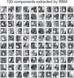
Listing 6.15. Representing the hidden units graphically

plt.figure(figsize=(4.2, 4))
for i, comp in enumerate(rbm.components_):
    #print(i)
    #print(comp)
    plt.subplot(10, 10, i + 1)
    plt.imshow(comp.reshape((8, 8)), cmap=plt.cm.gray_r,interpolation='nearest')
    plt.xticks(())
    plt.yticks(())

plt.suptitle('100 components extracted by RBM', fontsize=16)
plt.subplots_adjust(0.08, 0.02, 0.92, 0.85, 0.08, 0.23)
plt.show()

In our RBM, we have 100 hidden nodes and 64 visible units, because this is the size of the images being used. Each square in figure 6.14 is a grayscale interpretation of the weights between that hidden component and each visible unit. In a sense, each hidden component can be thought of as recognizing the image as given previously. In the pipeline, the logistic regression model then uses the 100 activation probabilities (P(h_j=1|v=image) for each j) as its input; thus, instead of doing logistic regression over 64 raw pixels, it’s performed over 100 inputs, each having a high value when the input looks close to the ones provided in figure 6.14. Going back to the first section in this chapter, you should now be able to see that we’ve created a network that has automatically learned some intermediate representation of the numbers, using a RBM. In essence, we’ve created a single layer of a deep network! Imagine what could be achieved with deeper networks and multiple layers of RBMs to create more intermediate representations!

6.6. Summary

• We provided you a whistle-stop tour of neural networks and their relationship to deep learning. Starting with the simplest neural network model, the MCP model, we moved on to the perceptron and discussed its relationship with logistic regression.
• We found that it’s not possible to represent nonlinear functions using a single perceptron, but that it’s possible if we create multilayer perceptrons (MLP).
• We discussed how MLPs are trained through backpropagation—and the adoption of differentiable activation functions—and provided you with an example whereby a non-linear function is learned using backpropagation in PyBrain.
• We discussed the recent advances in deep learning: specifically, building multiple layers of networks that can learn intermediate representations of the data.
• We concentrated on one such network known as a Restricted Boltzmann Machine, and we showed how you can construct the simplest deep network over the digits dataset, using a single RBM and a logistic regression classifier.